3.5.3. PID Module
Note
For now this module is not compatible with PyMoDAQ 4. Please use the PyMoDAQ 3.6.8 version, as mentioned latter in this documentation. We are currently working on to update the PID extension.
3.5.3.1. Introduction
This documentation is complementary to the video on the module :
https://www.youtube.com/watch?v=u8ifY4WqQEA
The PID module is useful if you would like to control a parameter of a physical system (a temperature, the length of an interferometer, the beam pointing of a laser…). In order to achieve this, you need a set of detectors to read the current state of the system, an interpretation of this reading, and a set of actuators to perform the correction.
Note
Notice that the speed of the corrections that can be achieved with this module are inherently limited below 100 Hz, because the feedback system uses a computer. If you need a faster correction, you should probably consider an analogic solution.
3.5.3.1.1. First example: a boiler
Let consider this physical system. Some water is put in a jar, let say we want to keep the temperature of the water to 40°C, this is our setpoint. The system is composed of a heating element (an actuator), and a thermometer (a detector).
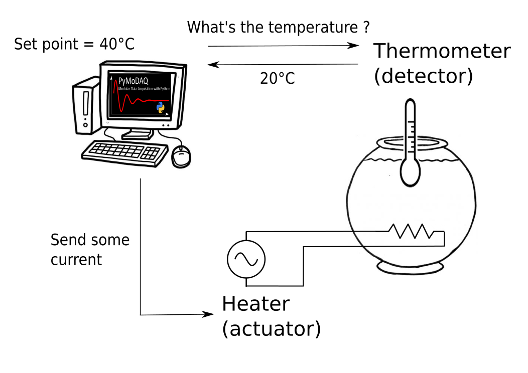
Fig. 3.38 The boiler system.
The control of the heater and the thermometer is a prerequisite to achieve the control of the temperature, but we also need a logic. For example:
if T - T_setpoint < 5°C then heater is ON
if T - T_setpoint > 5°C then heater is OFF
With this logic, when the hot water will have dissipated enough energy in its environment to reach 35°C, the heater will be switch on to heat it up to 45°C and then switch off. The temperature of the water will then be oscillating approximatelly around 40°C.
The difference between the setpoint and the current value of the control parameter, here T - T_setpoint, is called the error signal.
3.5.3.1.2. The PID Model
Depending on the system you want to control, there will be a different number of actuators or detectors, and a different logic. For example, if you want to control the pointing of a laser on a camera, you will need a motorized optical mount to hold a mirror with two actuators that control the tip and tilt axes, what we call a beam steering system. The way you calculate your error signal will be different: you will need a way to define the center of the laser beam on the camera, like the barycenter of the illuminated pixels, and the error signal will be a 2D vector, one for the vertical and one for the horizontal direction.

Fig. 3.39 The beam steering scheme.
Another exemple consists it propagating a continuous laser in the two arms of an interferometer to produce an interference pattern. The phase of the fringes depending on the difference in the arms’ lengths, it is possible to retrieve an error signal from this interference pattern to lock the interferometer, or even to sweep its length while it is locked.
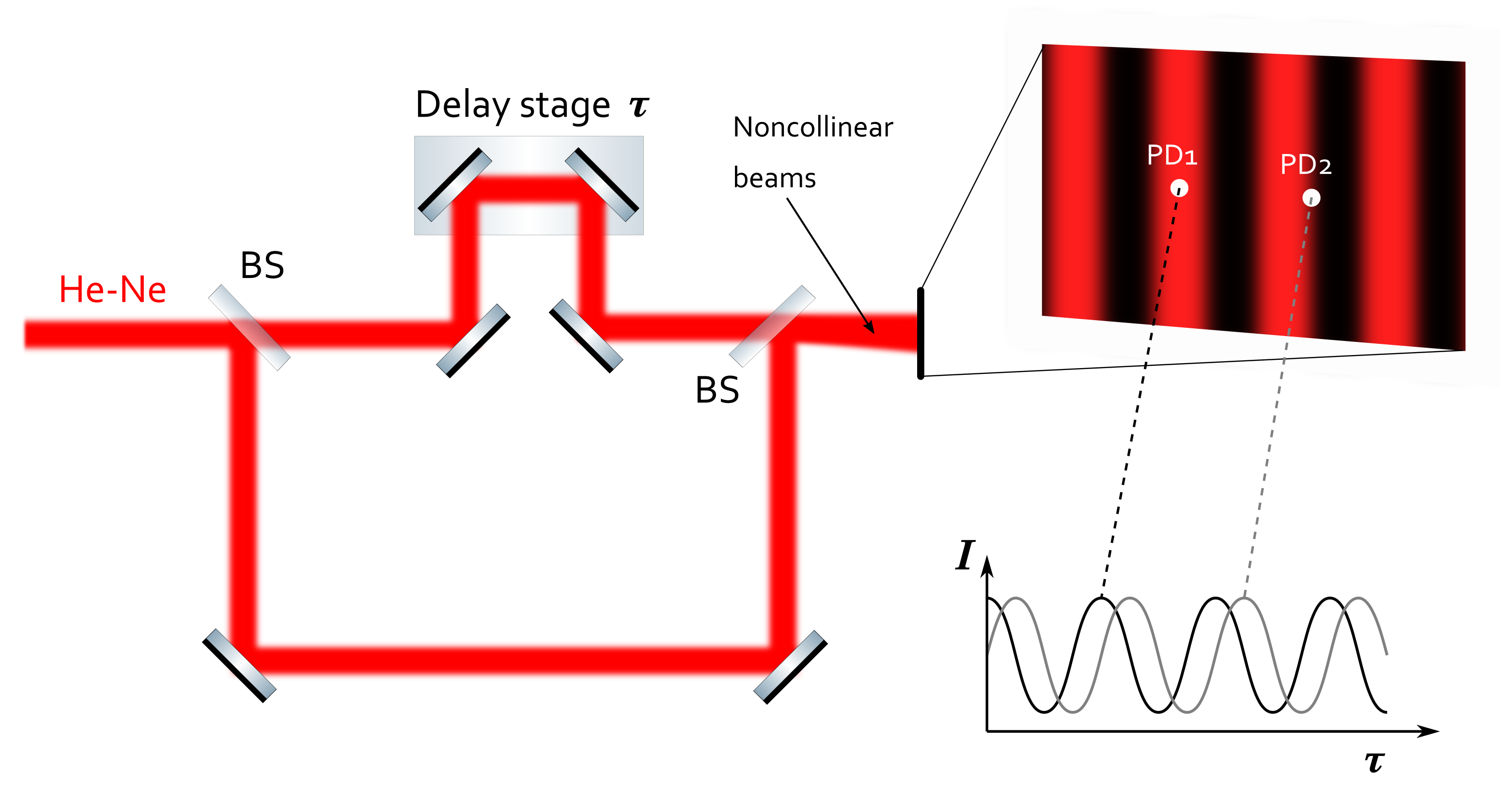
Fig. 3.40 The interferometer scheme.
The PID Model is a configuration of the PID module which depends on the physical system we want to control. It contains:
the number and the dimensionality of the required detectors
the number of actuators
the number of setpoints
the logic to calculate the error signal from the detectors’ signals
A PID model is associated to each different physical system we want to control.
3.5.3.2. Demonstration with a virtual beam steering system
Lucky you, you do not need a real system to test the PID module! A computer and an internet connection are enough. For our demonstration, we will install some mock plugins that simulate a beam steering system.
Let us start from scratch, we follow the installation procedure of PyMoDAQ that you can find in the installation page: https://pymodaq.cnrs.fr/en/latest/usage/Installation.html
We suppose that you have Miniconda3 or Anaconda3 installed.
In a console, first create a dedicated environment and activate it
conda create -n mock_beam_steering python=3.8
conda activate mock_beam_steering
Install PyMoDAQ with the version that have been tested while writing this documentation
pip install pymodaq==3.6.8
and the Qt5 backend
pip install pyqt5
We also need to install (from source) another package that contains all the mock plugins to test the PID module. This step is optional if you wish to use the PID module with real actuators and detectors.
pip install git+https://github.com/PyMoDAQ/pymodaq_plugins_pid.git
3.5.3.2.1. Preset configuration
Launch a dashboard
dashboard
Note
If at this step you get an error from the console, try to update to a newest version of the package “tables”, for instance pip install tables==3.7 and try again to launch a dashboard.
In the main menu go to
Preset Modes > New Preset
Let us choose a name, for example preset_mock_beam_steering.
Under the Moves section add two actuators by selecting BeamSteering in the menu, and configure them as follow. The controller ID parameter could be different from the picture in your case. Let this number unchanged for the first actuator, but it is important that all the two actuators and the detector have the same controller ID number. It is also important that the controller status of the first actuator be Master, and that the status of the second actuator and the detector be Slave. (This configuration is specific to the demonstration. Underneath the actuators and the detector share a same virtual controller to mimic a real beam steering system, but you do not need to understand that for now!)
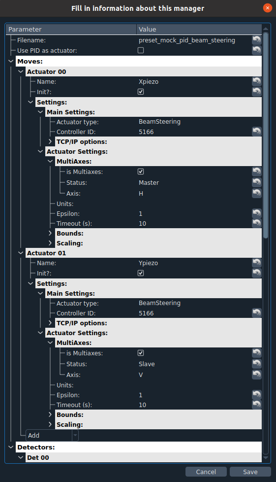
Fig. 3.41 The mock actuators configuration.
Now, add a 2D detector by selecting DAQ2D/BeamSteering in the menu, and configure it as follow
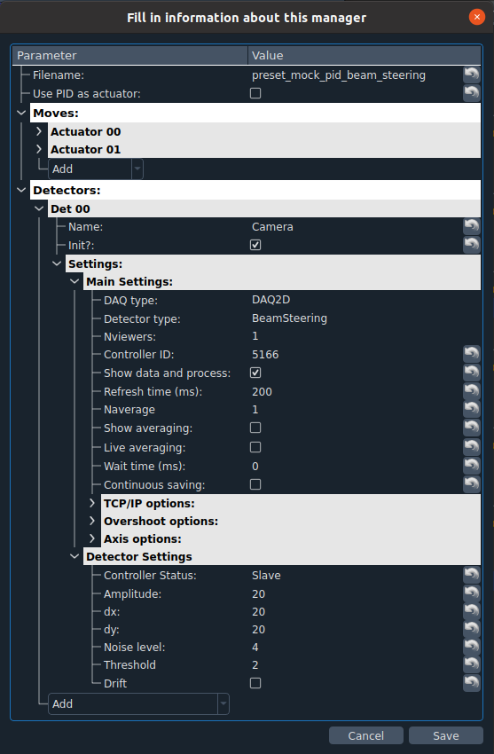
Fig. 3.42 The mock camera configuration.
and click SAVE.
Back to the dashboard menu
Preset Modes > Load preset > preset_mock_beam_steering
Your dashboard should look like this once you have grabbed the camera and unwrapped the option menus of the actuators.
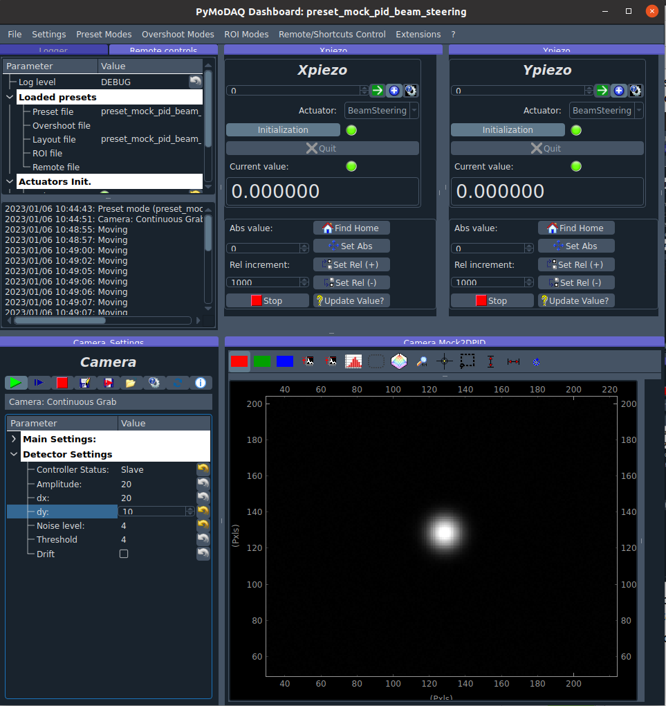
Fig. 3.43 The dashboard after loading the preset.
If you now try a relative move with Xpiezo or Ypiezo, you will see that the position of the laser spot on your virtual camera is moving horizontally or vertically, as if you were playing with a motorized optical mount.
Our mock system is now fully configured, we are ready for the PID module!
3.5.3.2.2. PID module
The loading of the PID module is done through the dashboard menu
Extensions > PID Module
It will popup a new window, in Model class select PIDModelBeamSteering and (1) initialize the model.
Configure it as follow:
camera refresh time (in the dashboard) = 200 ms
PID controls/sample time = 200 ms
PID controls/refresh plot time = 200 ms
threshold = 2
Then (2) intialize the PID and (3) start the PID loop with the PLAY button. Notice that at this stage the corrections are calculated, but the piezo motors are not moving. It is only when you will (4) untick the PAUSE button that the corrections will be applied.
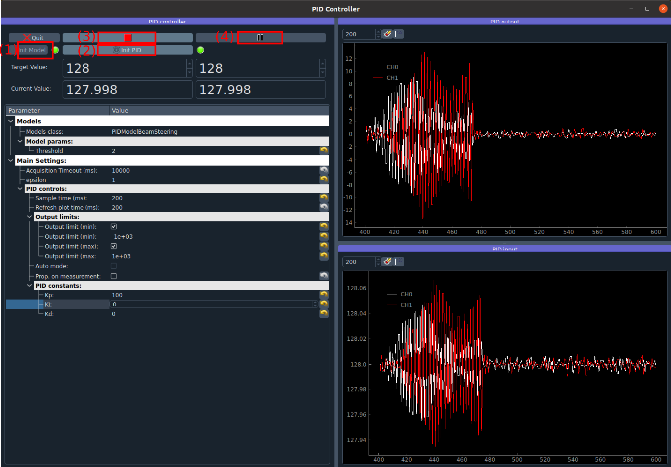
Fig. 3.44 The PID module interface.
3.5.3.2.3. PID configuration
Output limits
The output limits are here mainly to prevent the feedback system to send crazy high corrections and move our beam out of the chip.
If we put them too low, the feedback system will only send tiny corrections, and it will take a long time to correct an error, or if we change the setpoint.
If we increase them, then our system will be able to move much faster.
The units of the output limits are the same as the piezo motors, let say in microns. Put an output limit to +500 means “If at any time the PID outputs a correction superior to 500 microns, then only correct 500 microns.”
The output limits are not here to slow down the correction, if we want to do that we can decrease the proportional parameter (see next section). They are here to define what we consider as a crazy correction.
To define them we can pause the PID loop and play manually with the piezo actuators. We can see that if we do a 10000 step, we almost get out of the chip of the camera, thus an output limit of 1000 seems reasonable.
If we do a big change of setpoint and see that every step of the piezo corresponds to the output limit we configured, then it means the corrections are saturated by the output limits.
Configuring the PID parameters
The proportional, integral, derivative parameters of the PID filter, respectively Kp, Ki and Kd, will dictate the behavior of the feedback system.
Stay at a fixed position while the correction loop is closed, and start with Kp = 1, Ki = 0, Kd = 0. Then change the setpoint to go close to an edge of the camera. We see that the system is doing what it is supposed to do: the beam goes to the setpoint… but veeeeeeeeeeeeery slowly. This is not necessarily bad. If your application does only need to keep the beam at a definite position (e.g. if you inject an optical fiber), this can be a good configuration. If we take a look at the PID input display, which is just the measured position of the beam on the chip in pixel, we can see that reducing Kp will decrease the fluctuations of the beam around the target position. Thus a low Kp can increase the stability of your pointing.
Let say now that we intend to move regularly the setpoint. We need a more reactive system. Let us increase progressively the value of Kp until we see that the beam start to oscillate strongly around the target position (this should happen for Kp close to 200 - 300). We call this value of Kp the ultimate gain. Some heuristic method says that dividing the ultimate gain by 2 is a reasonable value for Kp. So let us take Kp = 100.
We will not go further in this documentation about how to configure a PID filter. For lots of applications, having just Kp is enough. If you want to go further you can start with this Wikipedia page: https://en.wikipedia.org/wiki/PID_controller.
3.5.3.2.4. Automatic control of the setpoints
Let us imagine now that we want to use this beam to characterize a sample, and that we need a long acquisition time at each position of the beam on the sample to perform our measurement. Up to now our feedback system allows to keep a stable position on the sample, which is nice. But it would be even better to be able to scan the surface of the sample automatically rather than moving the setpoints manually. That is the purpose of this section!
In order to do that, we will create virtual actuators on the dashboard that will control the setpoints of the PID module. Then, PyMoDAQ will see them as standard actuators, which means that we will be able to use any of the other modules, and in particular, perform any scan that can be configured with the DAQ_Scan module.
Preset configuration
Start with a fresh dashboard, we have to change a bit the configuration of our preset to configure this functionality. Go to
Preset Modes > Modify preset
and select the one that we defined previously. You just need to tick Use PID as actuator and save it.
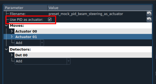
Fig. 3.45 Configuration of the preset for automatic control of the setpoints.
Moving the setpoints from the dashboard
Load this new preset. Notice that it now automatically loaded the PID module, and that our dashboard got two more actuators of type PID named Xaxis and Yaxis. If you change manually the position of those actuators, you should see that they control the setpoints of the PID module.
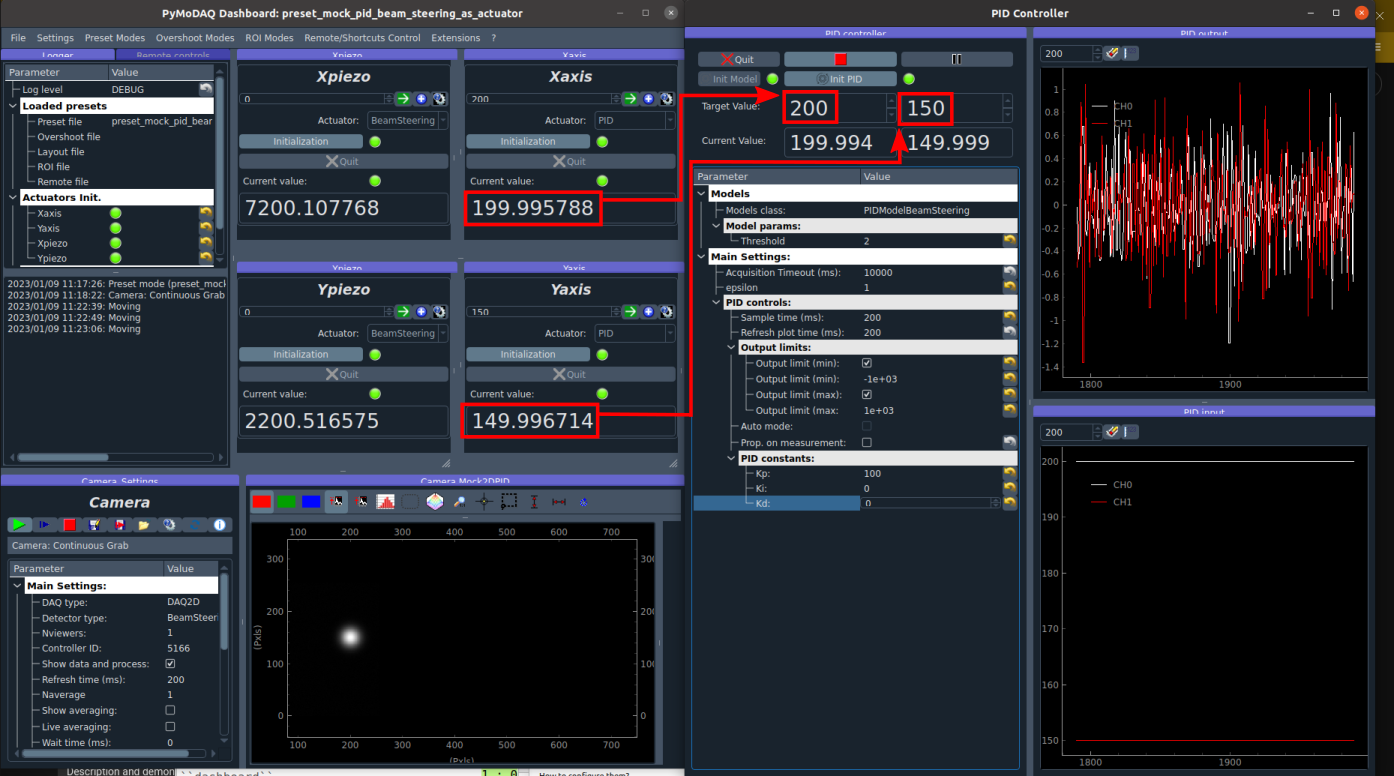
Fig. 3.46 Virtual actuators on the dashboard control the setpoints of the PID module.
Moving the setpoints with the DAQ Scan module
Those virtual actuators can be manipulated as normal actuators, and you can ask PyMoDAQ to perform a scan of those guys! Go to
Extensions > Do scans
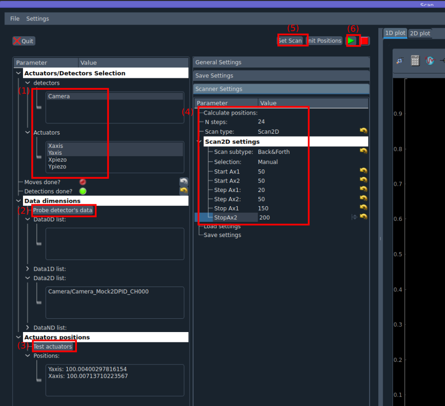
Fig. 3.47 Configuration of a scan with the DAQ_Scan module.
Some popup windows will ask you to name your scan. This is not important here. Configure the scan as follow
Select Camera, Xaxis, Yaxis (maintain Ctrl command to select several actuators)
Click Probe detector’s data
Click Test actuators and select a position at the center of the camera
Define a 2D scan as follow. Notice that Ax1 (associated to the Xaxis) corresponds to the main loop of the scan: its value is changed, then all the values of Ax2 are scanned, then the value of Ax1 is changed, and so on…
Set scan
Start and look at the camera
The beam should follow automatically the scan that we have defined. Of course in this demonstration with a virtual system, this sounds quite artificial, but if you need to perform stabilized scans with long acquisition times, this feature can be very useful!
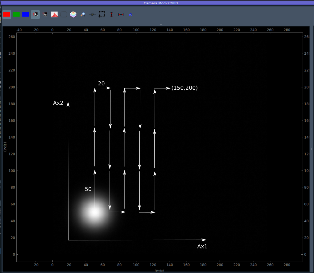
Fig. 3.48 Movement of the beam on the camera with a scan of the setpoints.
3.5.3.3. How to write my own PID application?
3.5.3.3.1. Package structure for a PID application
To write your own PID application, you should create a package with a similar structure as a standard pymodaq_plugins_xxx package. There are few modifications. Let us have a look at the pymodaq_plugins_pid.
Notice there is a models folder next to the hardware folder, at the root of the package. This folder will contains the PID models.
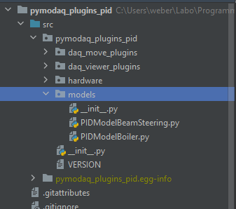
Fig. 3.49 Structure of a package containing PID models.
Then python will be able to probe into those as they have been configured as entry points during installation of the package. You should check that those lines are present in the setup.py file of your package.

Fig. 3.50 Declaration of entry points in the setup.py file.
This declaration allows PyMoDAQ to find the installed models when executing the PID module. Internally, it will call the get_models method that is defined in the daq_utils.
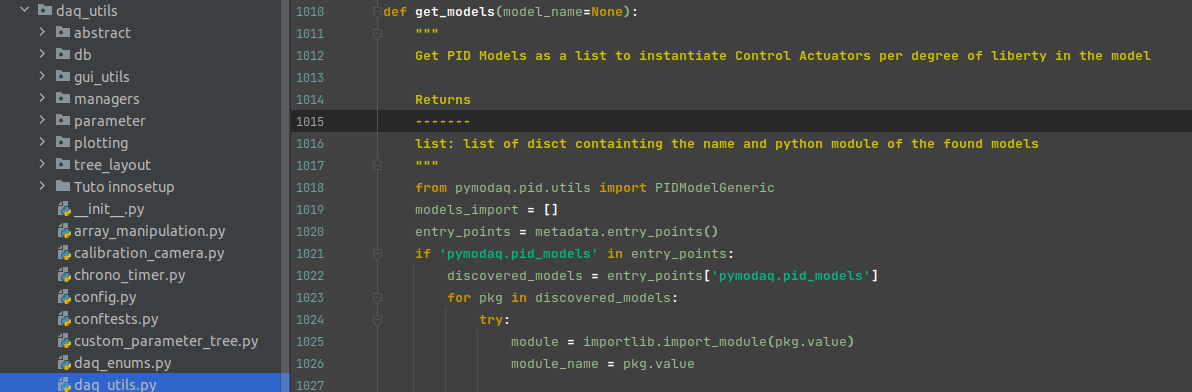
Fig. 3.51 The get_models method in the daq_utils.
In order to use the PID module for our specific physical system, we need:
A set of detector and actuator plugins that is needed to stabilize our system.
A PID model to implement the logic that is needed to translate the detectors’ signals into a correction.
3.5.3.3.2. Detector/actuator plugins
In the beam steering example, this corresponds to one actuator plugin (if you use the same motor model for horizontal and vertical axis), and a camera plugin.
The first thing to do is to check the list of readily available plugins.
The easy scenario is that you found that the plugins for your hardware are already developped. You then just have to test if they properly move or make an acquisition with the DAQ Move and DAQ Viewer modules. That’s it!
If there is no plugin developped for the hardware you want to use, you will have to develop your own. Don’t panic, that’s quite simple! Everything is explained in the Plugins section of the documentation, and in this video. Moreover, you can find a lot of examples for any kind of plugins in the list given above and in the GitHub repository of PyMoDAQ. If at some point, you stick on a problem, do not hesite to raise an issue in the GitHub repository or address your question to the mailing list pymodaq@services.cnrs.fr.
Note
It is not necessary that the plugins you use are declared in the same package as your model. Actually a model is in principle independent of the hardware. If you use plugins that are declared in other packages, you just need them to be installed in your python environment.
3.5.3.3.3. How to write a PID model?
Naming convention
Similarly to plugins, there exist naming conventions that you should follow, so that PyMoDAQ will be able to parse correctly and find the classes and the files that are involved.
The name of the file declaring the PID model should be named PIDModelXxxx.py
The class declared in the file should be named PIDModelXxxx
Number of setpoints and naming of the control modules
The number of setpoints, their names, and the naming of the control modules are declared at the begining of the class declaration. It is important that those names are reported in the preset file associated to the model. We understand now that those names are actually set in the PID model class.
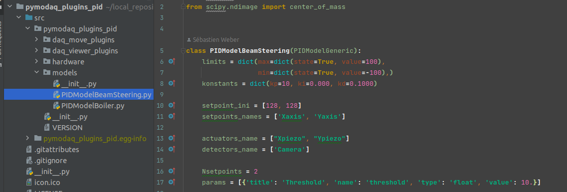
Fig. 3.52 Configuration of a PID model.
The required methods of a PID model class
There are two required methods in a PID model class:
convert_input that will translate the acquisitions of the detectors into an understandable input for the PID filter (which is defined in an external package).
convert_output that will translate the output of the PID filter(s) into an understandable order for the actuators.
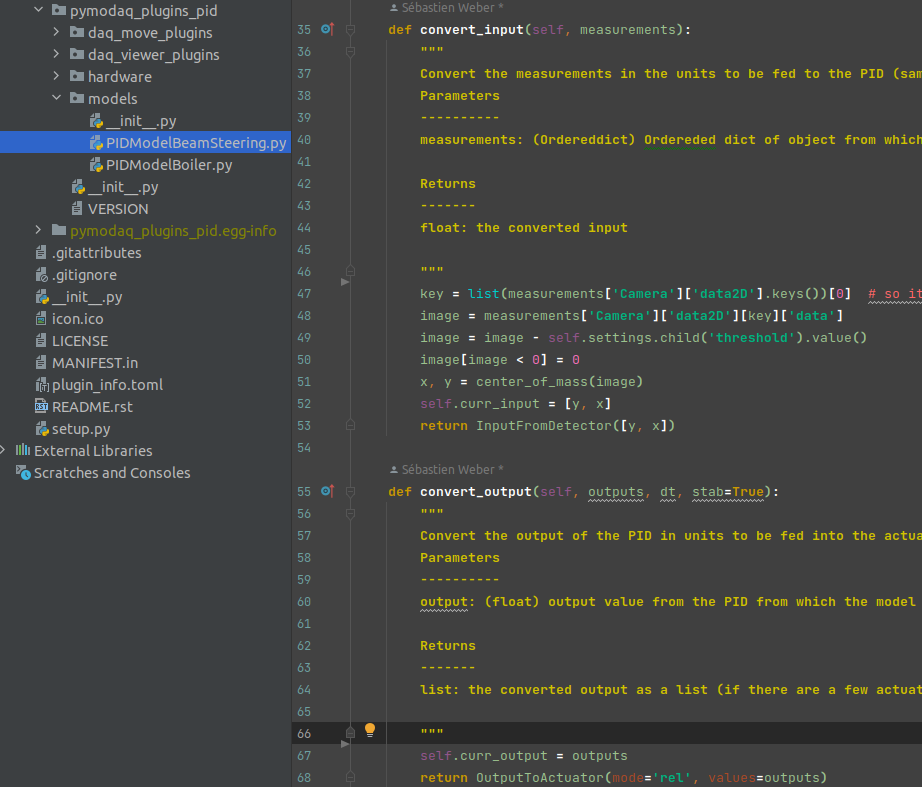
Fig. 3.53 The important methods of a PID model class.
In this example of the PIDModelBeamSteering, the convert_input method get the acquisition of the camera, remove the threshold value defined by the user through the UI (this is to remove the background noise), calculate the center of mass of the image, and send the coordinates as input to the PID filter.
Note
The PID filter is aware of the setpoints values, thus you just have to send him absolute values for the positioning of the system. He will calculate the difference himself.
As for the convert_output method, it only transferts the output of the PID filter directly as relative orders to the actuators.
Note
The output of the PID filter is a correction that is relative to the current values of the actuators.
That’s it!
Note
In this example, there is actually no other methods defined in the model, but you can imagine more complex systems where, for example, the translation from the detectors acquisitions to the input to the filter would need a calibration scan. Then you will probably need to define other methods. But, whatever it is, all the logic that is specific to your system should be defined in this class.
If you want to go deeper, the next section is for you!
3.5.3.4. PID module internals
This section is intended for the advanced user that intend to develop its custom application based on the PID module, or the one that is simply curious about the PID module internals. We will try to introduce here the main structure of the module, hoping that it will help to graps the code more easily :)
3.5.3.4.1. Files locations
The files regarding the PID module are stored in the /src/pymodaq/pid/ folder which contains:
utils.py which defines some utility classes, and in particular the PIDModelGeneric class from which all PID models inherit.
daq_move_PID.py which defines a virtual actuator that control the setpoint of the PID module. This is useful for example if the user wants to scan the control parameter while it is locked.
pid_controller.py. It is the core file of the module that defines the DAQ_PID and the PIDRunner classes that will be presented below.
3.5.3.4.2. Packages
PyMoDAQ/pymodaq_plugins_pid This package contains some mock plugins and models to test the module without hardware. It is for development purposes and thus optional.
PyMoDAQ/pymodaq_pid_models This package stores the PID models that have already been developped. Better to have a look before developping its own!
3.5.3.4.3. General structure of the module

Fig. 3.54 The structure of the PID module.
The DAQ_PID class is the main central class of the module. It manages the initialization of the program: settings of the user interface, loading of the PID model, instanciation of the PIDRunner class… It also makes a bridge between the user, who acts through the UI, and the PIDRunner class, which is the one that is in direct relation with the detectors and the actuators.
Since each of those classes is embbeded in a thread, the communication between them is done through the command_pid_signal and the queue_command method.
The PIDRunner class is created and configured by the DAQ_PID at the initialization of the PID loop. It is in charge of synchronizing the instruments to perform the PID loop.
A PIDModel class is defined for each physical system the user wants to control. Here are defined the actuator/detector modules involved, the number of setpoints, and the methods to convert the information received from the detectors as orders to the actuators to perform the desired control.
3.5.3.4.4. The PID loop
The conductor of the PID loop is the PIDRunner, in particular the start_PID method. The workflow for each iteration of the loop can be mapped as in the following figure.

Fig. 3.55 An iteration of the PID loop.
The starting of the PID loop is triggered by the user through the PLAY button.
The PIDRunner will ask the detector(s) to start an acquisition. When all are done, the wait_for_det_done method will send the data (det_done_datas) to the PIDModel class.
A PIDModel class should be defined for each specific physical system the user wants to control. Here are defined how much detectors/actuators are involved, and how the information sent by the detector(s) should be converted as orders to the actuators (output_to_actuators) to reach the targeted position (the setpoint). The PIDModel class is thus an iterface between the PID class and the detectors/actuators. The important methods of those classes are convert_input, which will convert the detectors data to an input for the PID object, and the convert_output method which will translate the output of the PID object to the actuators.
The PID class is defined in an external package (simple_pid: https://github.com/m-lundberg/simple-pid). It implements a pid filter. The tunnings (Kp, Ki, Kd) and the setpoint are configured by the user through the user interface. From the input, which corresponds to the current position of the system measured by the detectors, it will return an output that corresponds to the order to send to the actuators to stabilize the system around the setpoint (given that the configuration has been done correctly). Notice that the input for the PID object should be an absolute value, and not a relative value from the setpoint. The setpoint is entered as a parameter of the object so it can make the difference itself.