3.7. Useful Modules
3.7.1. Introduction
Utility modules are used within each main modules of PyMoDAQ but can also be used as building blocks for custom application. In that sense, all Plotting Data and even DAQ Viewer and DAQ Move can be used as building blocks to control actuators and display datas in a custom application.
3.7.2. Module Manager
The module manager is an object used to deal with:
Selection of actuators and detectors by a user (and internal facilities to manipulate them, see the API when it will be written…)
Synchronize acquisition from selected detectors
Synchronize moves from selected actuators
Probe as lists all the datas that will be exported by the selected detectors (see Fig. 3.84)
Test Actuators positioning. Clicking on test_actuator will let you enter positions for all selected actuators that will be displayed when reached
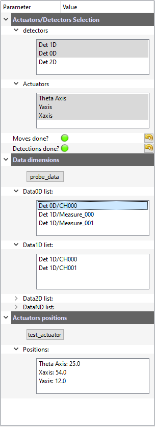
Fig. 3.84 The Module Manager user interface with selectable detectors and actuators, with probed data feature and actuators testing.
3.7.2.1. Scan Selector
Scans can be specified manually using the Scanner Settings (explained above). However, in the case of a scan using 2 DAQ_Move modules, it could be more convenient to select an area using a rectangular ROI within a 2D viewer. Various such viewers can be used. For instance, the viewer of a camera (if one think of a camera in a microscope to select an area to cartography) or even the DAQ_Scan 2D viewer. Sometimes it could also be interesting to do linear sections within a 2D phase space (let’s say defined by the ranges of 2 DAQ_Moves). This defines complex tabular type scan within a 2D area, difficult to set manually. Fig. 3.34 displays such sections within the DAQ_Scan viewer where a previous 2D scan has been recorded. The user just have to choose the correct selection mode in the scanner settings, see Fig. 3.85, and select on which 2D viewer to display the ROI (From Module option).
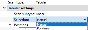
Fig. 3.85 In the scanner settings, the selection entry gives the choice between Manual selection of from PolyLines (in the case of 1D scans) or From ROI in the case of 2D scans.
3.7.2.2. Module Manager
This module is made so that selecting actuators and detectors for a given action is made easy. On top of it, there are features to test communication and retrieve infos on exported datas (mandatory fro the adaptive scan mode) or positioning. Internally, it also features a clean way to synchronize detectors and actuators that should be set together within a single action (such as a scan step).
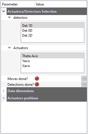
Fig. 3.86 User interface of the module manager listing detectors and actuators that can be selected for a given action.
3.7.3. H5Saver
This module is a help to save data in a hierachical hdf5 binary file through the pytables package. Using the H5Saver
object will make sure you can explore your datas with the H5Browser. The object can be used to: punctually save one set
of data such as with the DAQ_Viewer (see daq_viewer_saving_single), save multiple acquisition such as with the DAQ_Scan
(see Saving: Dataset and scans) or save on the fly with enlargeable arrays such as the Continuous Saving mode of the DAQ_Viewer.
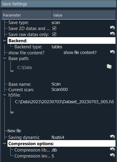
Fig. 3.87 User interface of the H5Saver module
On the possible saving options, you’ll find (see Fig. 3.87):
Save type:
Save 2D and above: True by default, allow to save data with high dimensionality (taking a lot of memory space)
Save raw data only: True by default, will only save data not processed from the Viewer’s ROIs.
backend display which backend is being used: pytables or h5py
Show file content is a button that will open the
H5Browserinterface to explore data in the current h5 fileBase path: where will be saved all the data
Base name: indicates the base name from which the actual filename will derive
Current scan indicate the increment of the scans (valid for DAQ_Scan extension only)
h5file: readonly, complete path of the saved file
Do Save: Initialize the file and logging can start. A new file is created if clicked again, valid for the continuous saving mode of the
DAQ_ViewerNew file is a button that will create a new file for subsequent saving
Saving dynamic is a list of number types that could be used for saving. Default is float 64 bits, but if your data are 16 bits integers, there is no use to use float, so select int16 or uint16
Compression options: data can be compressed before saving, using one of the proposed library and the given value of compression [0-9], see pytables documentation.
3.7.4. Preset manager
The Preset manager is an object that helps to generate, modify and save preset configurations of DashBoard. A preset is a set of actuators and detectors represented in a tree like structure, see Fig. 3.88.
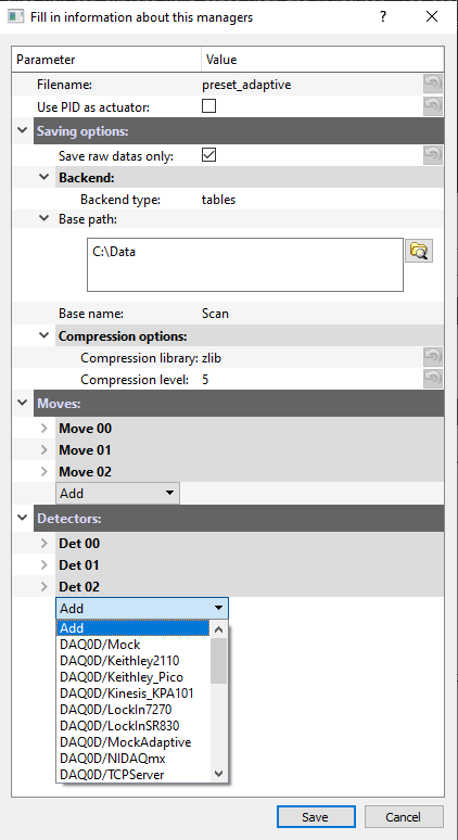
Fig. 3.88 An example of a preset creation named preset_adaptive containing 3 DAQ_Move modules and 3 detector modules and just about to select a fourth detector from the list of all available detector plugins.
Each added module load on the fly its settings so that one can set them to our need, for instance COM port selection, channel activation, exposure time… Every time a preset is created, it is then loadable. The init? boolean specifies if the Dashboard should try to initialize the hardware while loading the module in the dashboard.
3.7.5. Overshoot manager
The Overshoot manager is used to configure safety actions (for instance the absolute positioning of one or more actuators, such as a beam block to stop a laser beam) when a detected value (from a running detector module) gets out of range with respect to some predefined bounds, see Fig. 3.89. It is configurable in the framework of the Dashboard module, when actuators and detectors have been activated. A file containing its configuration will be saved (with a name derived from the preset configuration name and will automatically be loaded with its preset if existing on disk)
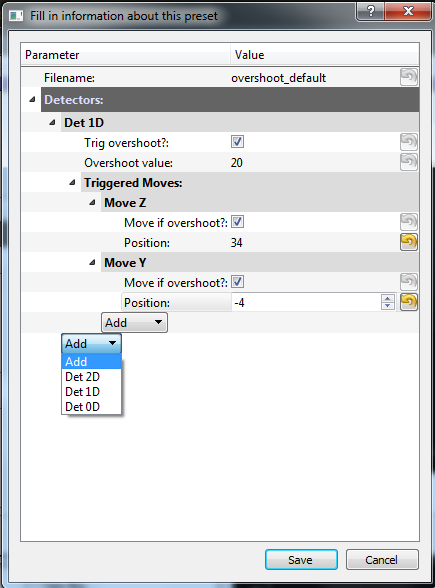
Fig. 3.89 An example of an overshoot creation named overshoot_default (and corresponding xml file) containing one listening detector and 2 actuators to be activated.
3.7.6. ROI manager
The ROI manager is used to save and load in one click all ROIs or Lineouts defined in the current detector’s viewers, see Fig. 3.90. The file name will be derived from the preset configuration file, so that at start up, it will automatically be loaded, and ROIs and Lineouts will be restored.
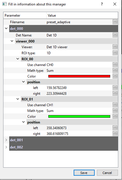
Fig. 3.90 An example of ROI manager modification named from the preset preset_adaptive (and corresponding xml file) containing all ROIs and lineouts defined on the detectors’s viewers.
3.7.7. DAQ_Measurement
In construction
3.7.9. Remote Manager
In construction
3.7.10. ChronoTimer
Fig. User Interface of the Chrono/Timer UI shows a user interface to be used for timing things. Not really part of PyMoDAQ but well could be useful (Used it to time a roller event in my lab ;-) )
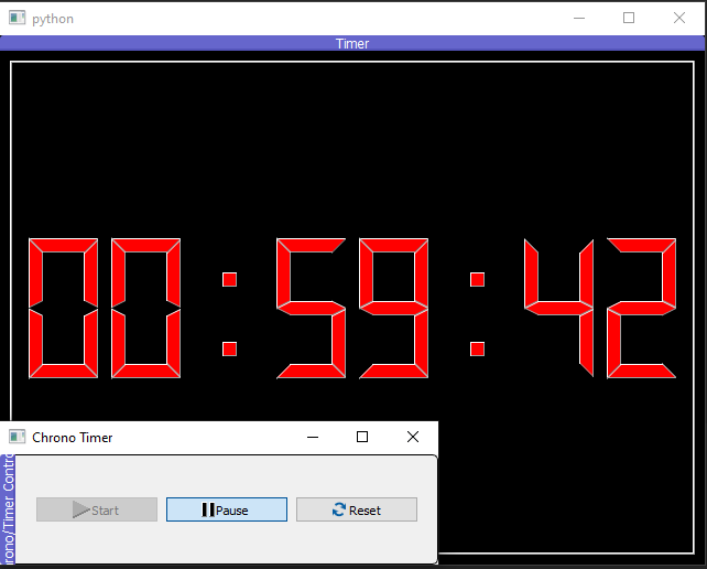
Fig. 3.91 User Interface of the Chrono/Timer UI