2.4. Data viewers

PyMoDAQ displays its data in data viewers. Each DAQ_Viewer uses one or several of them, depending on the dimensionality of the data sent by its instrument plugin. The same viewers are used everywhere in PyMoDAQ (scans, H5Browser, extensions…):

• Viewer0D, for scalars, plots their history;

• Viewer1D, for waveforms and any one dimensional data;

• Viewer2D, for images and any two dimensional data, either on a regular grid (uniform data) or not (spread data);

• ViewerND, for anything else: it combines the other viewers to explore the navigation and signal parts of the data, see DataWithAxes and signal/navigation axes.

When several data objects have to be displayed at once (a DataToExport), a ViewerDispatcher creates on the fly one dock with the adapted viewer for each of them. This is what the DAQ_Viewer and the DAQ_Scan do.

This page explains how to use the viewers from their toolbar: the crosshair, the Regions Of Interest (ROIs) that produce new data from the displayed ones, and the ROI select, a selection sent back to the instrument plugin. To plot your own data objects from a script or a notebook, see Plotting Data.

Note

The default state (checked or not) of most toolbar buttons can be set in the viewer section of the gui preferences, see Preferences files. For instance ROIselect = true in [viewer.viewer2D] makes the ROI select visible when a Viewer2D is created, and Nhistory in [viewer.viewer0D] sets the default history length of the Viewer0D.

2.4.1. Toolbars

2.4.1.1. Viewer0D

The Viewer0D plots the history of scalar data: each new value is added at the end of its curve, see Fig. 2.25.

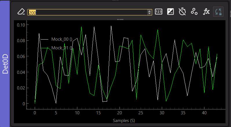
Fig. 2.25 A Viewer0D of the Dashboard showing the history of two channels.

Button	Action
	Clear the plot (the histories)
	Length of the history: the number of samples kept in the plot
	Display the last values as numbers in a side panel
	Display horizontal dashed lines at the min and max of each channel
	Use the timestamps of the data as horizontal axis, instead of the sample number
	Show the data as dots only (scatter)
	With two channels, plot one as a function of the other (XY mode, only shown with two channels)
	When checked (default), adding a new channel resets all the histories so that all curves share the same origin. Otherwise the existing curves keep their history

2.4.1.2. Viewer1D

The Viewer1D plots one or several waveforms against their axis, see Fig. 2.26.

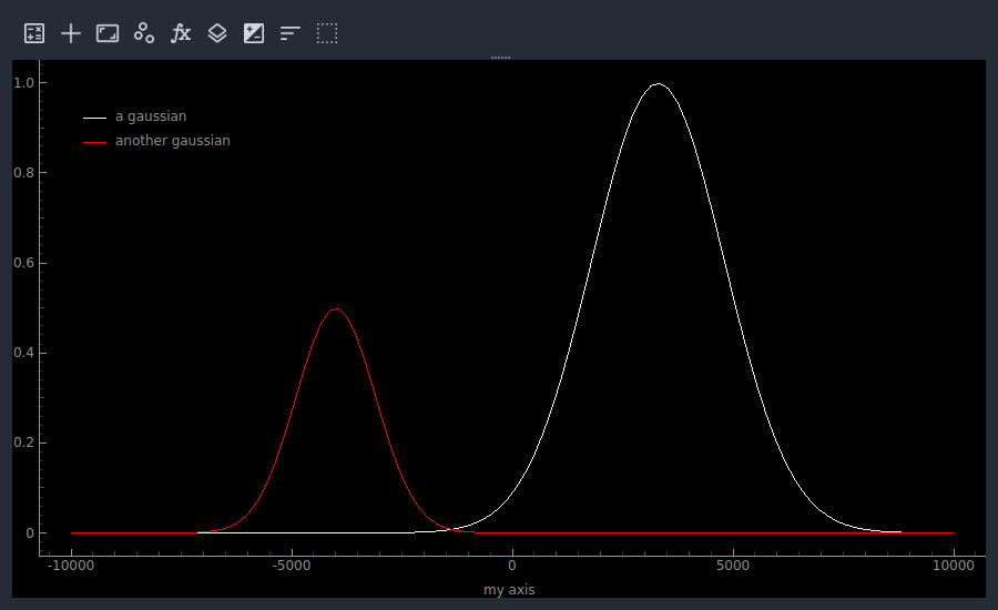
Fig. 2.26 A Viewer1D showing two waveforms. The legend gives the labels of the data, the axis its label and units.

Button	Action
	Show the ROI manager to define regions of interest on the waveforms, see Regions of interest
	Show the crosshair, see Crosshair
	Fix the horizontal/vertical aspect ratio
	Show the data as dots only (scatter)
	With two waveforms, plot one as a function of the other (XY mode, only shown with two waveforms)
	Keep an overlay (dashed line) of the current data
	Show the errors (if any) as an area around the curves
	Sort the data by ascending axis values (useful for non monotonous axes)
	Show the ROI select, see ROI select

2.4.1.3. Viewer2D

The Viewer2D plots images, see Fig. 2.27. When the data object holds several arrays, they are displayed as the red, green and blue layers of the image.

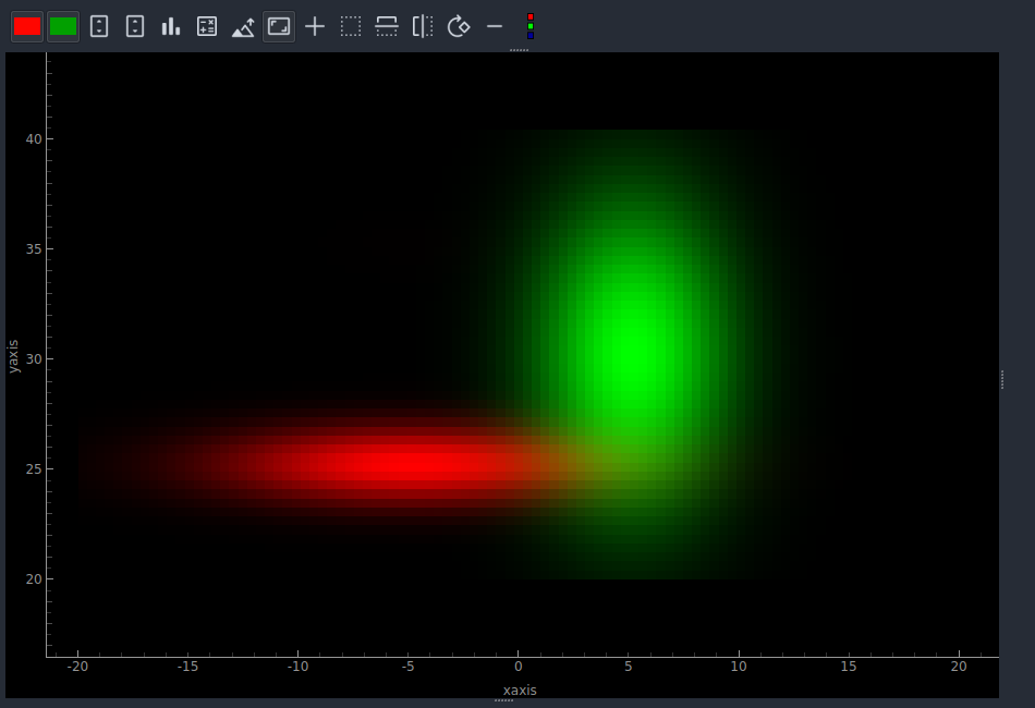
Fig. 2.27 A Viewer2D showing two arrays (red and green layers) of the same image.

Button	Action
	Show/hide the red, green or blue channel (one button per array of the data)
	Autoscale the color levels, between the min and max of the data or symmetrically around zero
	Show the histogram panel to set the color levels manually
	Show the ROI manager and the lineout panels, see Regions of interest
	Link the zoom of the lineout panels to the one of the image (shown with the ROI manager or the crosshair)
	Show an isocurve, whose level is set from the histogram
	Fix the aspect ratio to one
	Show the crosshair and its lineouts, see Crosshair
	Show the ROI select, see ROI select
	Flip the image up/down or left/right, or rotate it
	Display the opposite of the image
	Show/hide the legend

Images are displayed in the units of their axes: the coordinates read on the viewer (mouse position, crosshair, ROIs, ROI select) are given in these units, or in pixels when the data has no axes.

2.4.1.4. ViewerND

The ViewerND plots data that doesn’t fit in the other viewers: the data is split into a navigation part and a signal part (of dimension 0, 1 or 2), see DataWithAxes and signal/navigation axes. It is made of a navigation panel and a signal panel, each of them being a Viewer1D or Viewer2D (or several Viewer1D when there are more than two navigation axes), see Fig. 2.28. The signal panel shows the signal data indexed at the position of the crosshair of the navigation panel, the navigation panel shows the result of a math operation applied on the ROI of the signal panel for all navigation positions. The panel on the left displays the shape of the data and lets you change which axes are navigation or signal.

Fig. 2.28 A ViewerND showing 4D data with two navigation axes: a Viewer2D for the navigation (left) and one for the signal (right).

Button	Action
	Open a side window to control which axes are navigation axes
	Select the math operator applied on the signal ROI to compute the navigation data
	Add another signal plot showing the signal integrated over all the navigation axes, instead of the one indexed at the crosshair position

With spread data, all navigation axes are plotted in the same Viewer1D. The toolbars of the Viewer1D and Viewer2D panels are the ones described above.

2.4.2. Crosshair

The crosshair ( button) is a vertical line (Viewer1D) or a pair of lines (Viewer2D) that you can drag, or move with a double click on the plot. In a Viewer1D, its position (x) and the values of each trace at this position (y, separated by /) are printed in the toolbar, see Fig. 2.29. In a Viewer2D, its position and the value of each channel at this position are printed on the left of the toolbar, and it displays the lineouts of the image along its lines: the horizontal one below the image, the vertical one on its right, and the history of the value at its position in the bottom right corner, see Fig. 2.30.

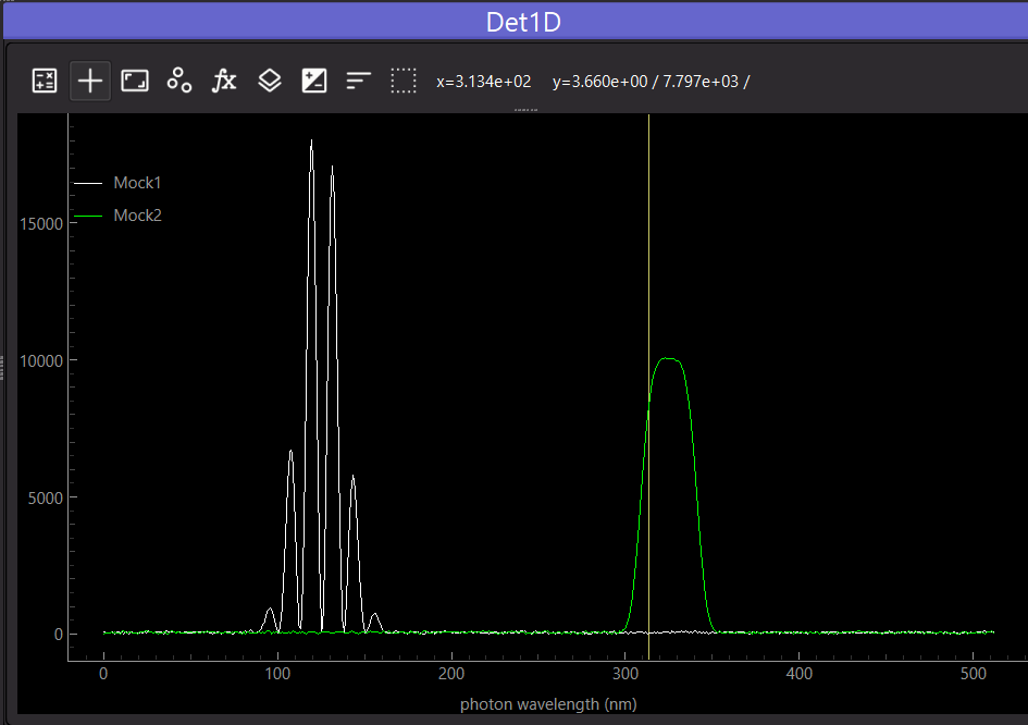
Fig. 2.29 A Viewer1D with the crosshair (yellow line). The toolbar prints its position and the value of the two traces at this position.

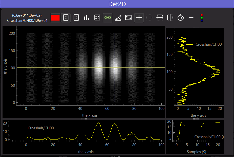
Fig. 2.30 A Viewer2D (one channel) with the crosshair and its horizontal, vertical and history lineouts. The top left of the toolbar prints its position and the value of the channel at this position.

Its position is sent to the instrument plugin each time it is moved, so that a plugin can use it (for instance to point a scanner to the selected position), see Reacting to the viewers: ROI select and crosshair.

2.4.3. Regions of interest

The ROI manager ( button) is a panel listing the ROIs of the viewer. In the Dashboard, it is shown in the ROIs dock, on the right of the detectors, see Fig. 2.31. Its title gives the detector and the viewer it belongs to, its buttons detach it as a separate window or close it (which unchecks the ROI button). Whether it starts docked or detached, and the horizontal or vertical layout of the dock, are set by the rois_as_popup and rois_dock_layout entries of the gui preferences (the layout can also be changed from the right-click menu of the dock).

Use the Add button of the panel to create a new ROI:

• in a Viewer1D, a ROI is a region along the axis, delimited by two draggable lines;

• in a Viewer2D, you can choose between a rectangular (RectROI), elliptical (EllipseROI) or circular (CircularROI) ROI, that you can move, resize and, for the rectangular one, rotate.

Each ROI has its own settings, also editable from the panel:

• Use channel: the data channel(s) (traces of a Viewer1D, red/green/blue arrays of a Viewer2D) the ROI applies to;

• Math type: the operation applied on the data within the ROI: mean, sum, std, max, min, or the position of a feature (argmax, argmin, argmean, argstd);

• its position and size, its color, and in 2D its type and angle.

Each ROI produces new data, computed every time the viewer receives data:

• in a Viewer1D, a scalar per ROI and channel, whose history is plotted in a panel below the waveforms;

• in a Viewer2D, the horizontal and vertical lineouts (Hlineout, Vlineout, the math operation applied along one direction of the ROI) and a scalar (Integrated, applied along both directions). They are plotted in the lineout panels: horizontal lineouts below the image, vertical lineouts on its right, and the history of the scalars in the bottom right corner, see Fig. 2.32.

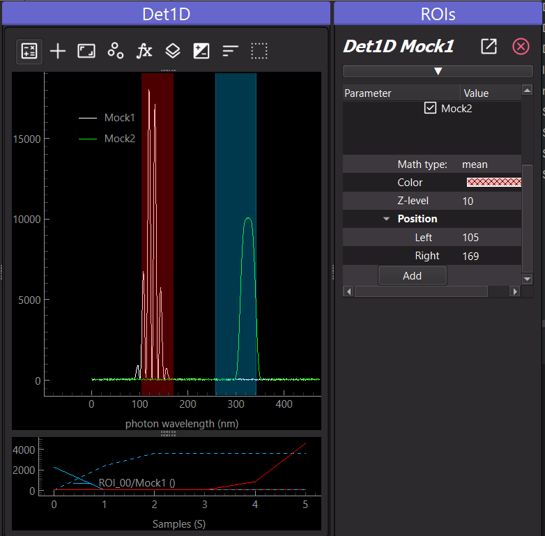
Fig. 2.31 A Viewer1D of the Dashboard with two ROIs, one on each trace. The bottom panel plots the history of their mean value. On the right, the ROIs dock shows the settings of the ROIs of this viewer.

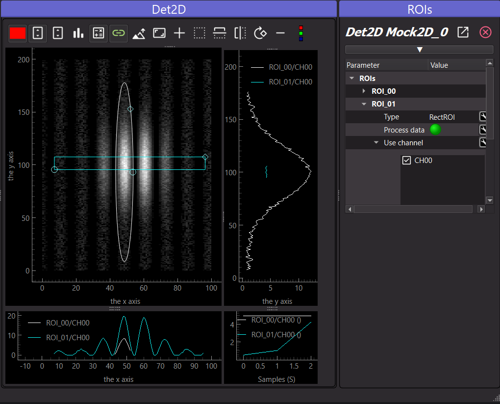
Fig. 2.32 A Viewer2D of the Dashboard with an elliptical (ROI_00) and a rectangular (ROI_01) ROI. Their horizontal lineouts are plotted below the image, their vertical lineouts on its right and the history of their integrated value in the bottom right panel. The ROIs dock shows the settings of ROI_01.

These data are sent along with the raw data of the DAQ_Viewer: they can be used by the extensions (DAQ_Scan, DAQ_Logger…) as any other data, and are saved in the h5 files unless the Save raw data only option is checked (see H5Saver).

The save and load buttons of the panel store or restore the ROIs of a viewer as an xml file (by default in the settings folder of the user .pymodaq folder). To save and restore the ROIs of all the detectors of an experiment at once, use the Dashboard ROI manager. With the restore_rois preference ([viewer] section of the pymodaq preferences), these ROIs are restored automatically each time the experiment is loaded.

2.4.4. ROI select

The ROI select ( button) is a single extra selection, independent of the ROI manager:

• in a Viewer1D, a region delimited by two draggable lines;

• in a Viewer2D, a rectangle, that you can move by dragging it and resize from its corner and side handles (it can’t be rotated). When shown, it covers the central part of the view, see Fig. 2.33.

It doesn’t produce any data by itself. Instead, each time you release it after moving or resizing it, its position and size are sent to the instrument plugin of the DAQ_Viewer (in the units of the viewer axes). What happens then depends on the plugin. Typical uses are:

• cropping the data emitted by the plugin to the selected area;

• setting a hardware ROI on a camera, to read only the selected pixels and increase the frame rate.

If a plugin doesn’t use it, moving the ROI select has no effect. To use it in your own plugin, see Reacting to the viewers: ROI select and crosshair.

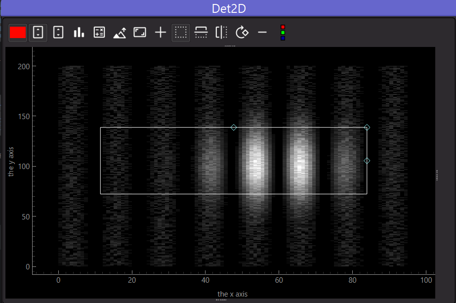
Fig. 2.33 A Viewer2D with the ROI select (white rectangle) shown. Its handles resize it, the selection is sent to the instrument plugin each time it is released.