2.3.2.2. DAQ Viewer

This module is to be used to interface any detector. It will display hardware settings and display data as exported by the hardware plugins (see Emission of data). The default detector is a Mock one (a kind of software based detector generating data and useful to test the program development). Other detectors may be loaded as plugins, see Instrument Plugins.

2.3.2.2.1. Introduction

The DAQ_Viewer interface is made of a toolbar and of one or more data viewers specific of the type of data to be acquired (see Data viewers). The settings of the module are displayed in a Settings dock that is shown or hidden from the toolbar. Fig. 2.19 displays a DAQ_Viewer started as a stand alone application (daq_viewer command) with a mock 2D detector.

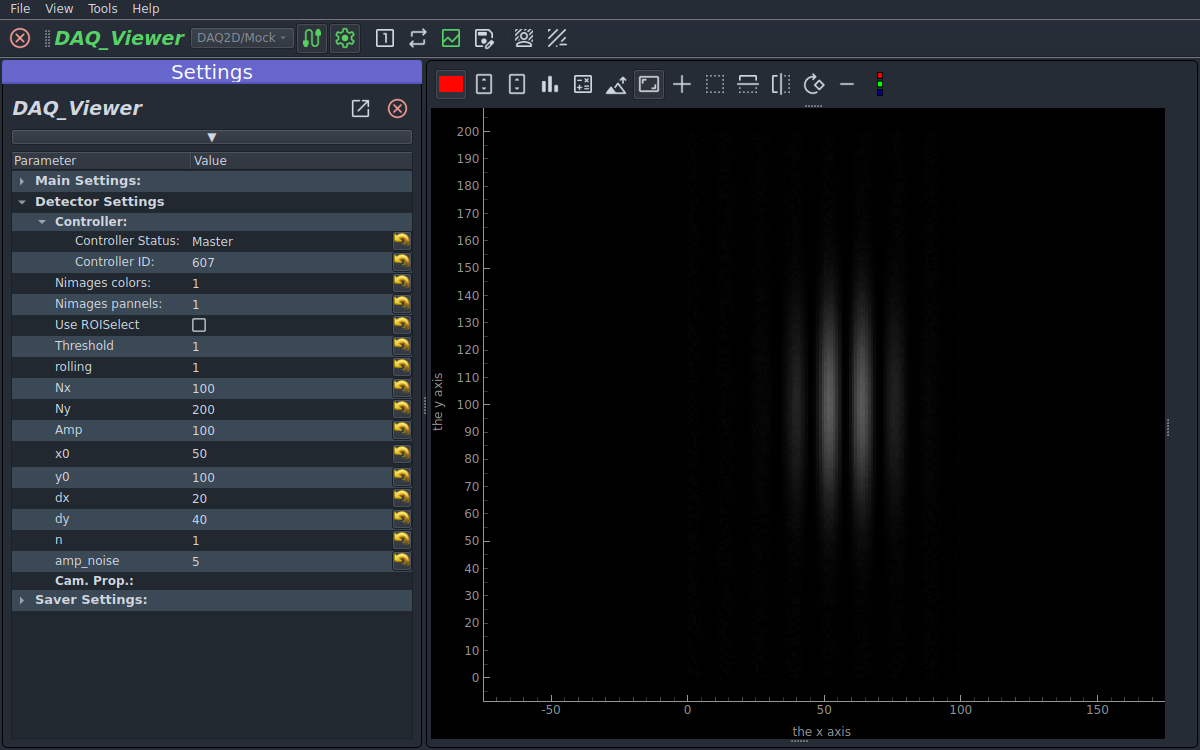
Fig. 2.19 A DAQ_Viewer with a mock 2D detector: toolbar on top, Settings dock on the left and a 2D data viewer on the right.

When the DAQ_Viewer is part of the Dashboard (see DashBoard), the same elements are displayed in the Dashboard: the toolbar and the data viewers in the module’s window, the settings in a Settings dock and the regions of interest in a ROIs dock. These docks can be detached from the window (Settings dock and other docks).

2.3.2.2.2. Toolbar

Fig. 2.20 The DAQ_Viewer toolbar once the detector is initialized.

The toolbar, Fig. 2.20, is where you choose and initialize the detector and trigger data acquisition. From left to right:

• Quit (red cross, stand alone application only): close the module and release the hardware.

• Name: title of the module. It turns green once the detector is initialized.

• Detector selection: the DAQ type/plugin drop-down list, see Hardware choice and initialization.

• / : initialize (or close) the selected detector. The icon is red when the detector is not initialized and green when it is.

• : show or hide the Settings dock, see Settings.

• : start a single acquisition (snap). Strongly advised for the first time data is acquired after initialization. The icon is red while the module is waiting for the data and green when the data has been received.

• : start (and stop, when clicked again) a continuous acquisition (grab).

• : reset the live averaging, only visible when Live averaging is activated, see Settings.

• : show or hide the data viewers, can be used to save screen space or to speed up the acquisition when the display is not needed.

• : save the current data in a h5 file, see Snapshots.

• : do a snap and keep the data as a background, see Background.

• : subtract the background from the displayed data.

All the toolbar actions are disabled until the detector is initialized (except the detector selection, the initialization and the show actions).

2.3.2.2.3. Hardware choice and initialization

Fig. 2.21 The toolbar before the initialization of the detector.

The DAQ type/plugin drop-down list (Fig. 2.21) lists the instrument plugins of type detector. They are sorted by the dimensionality of the data they are generating (DAQ2D for cameras, DAQ1D for waveforms, timeseries… and DAQ0D for detectors generating scalars such as powermeter, voltmeter…). Once a plugin is selected, the button starts the initialization using the values currently set in the Settings dock (so, if needed, set them before initializing). If the initialization is successful the name of the module and the initialization icon turn green and the other actions of the toolbar become available. Changing the detector is only possible while the module is not initialized.

2.3.2.2.3.1. Background

• : do a specific snap where the data will be internally kept as a background (and saved in a h5 file if you save data)

• : use the background previously taken to correct the displayed data (only the displayed ones, saved data are still the raw data). Un-check it to go back to the raw data.

2.3.2.2.4. Settings

The settings are displayed in the Settings dock, shown or hidden with the button. They are organized in three sections: the Main Settings (common to all detectors, UI and acquisition control), the Detector Settings (specific to the instrument plugin, see Instrument Plugins) and the Saver Settings (see Saver settings).

2.3.2.2.4.1. Main settings

Main settings refers to settings common to all instrument plugin. They are mostly related to the UI control.

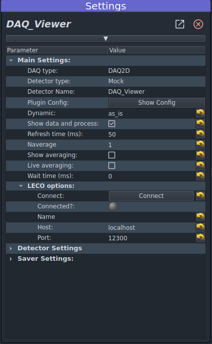
Fig. 2.22 Typical DAQ_Viewer Main settings.

• DAQ type: readonly string recalling the DAQ type used

• Detector type: readonly string recalling the selected plugin

• Detector Name: readonly string recalling the given name of the detector (from the experiment)

• Plugin Config: button displaying the configuration file of the plugin (if any)

• Dynamic: type of the data (as it is, or cast into a given type such as uint8, int16, float32…) in which the data will be displayed and saved. Default is as_is

• Show data and process: boolean for plotting (or not data in the data viewer)

• Refresh time (ms): used to slow down the refreshing of the display (but not of the eventual saving…)

• Naverage: integer to set in order to do data averaging, see Hardware averaging.

• Show averaging: in the case of software averaging (see Hardware averaging), if this is set to True, intermediate averaging data will be displayed

• Live averaging: show averaging must be set to False. If set to True, a live grab will perform non-stop averaging (current averaging value will be displayed just below, as N Live aver., and can be reset with the button). Could be used to check how much one should average, then set Naverage to this value

• Wait time (ms): Extra waiting time before sending data to viewer, can be used to cadence DAQ_Scan execution, or data logging

• LECO options: to connect the module to a LECO server (host, port and name of the module) and let other processes control it or receive its data, see LECO communication.

2.3.2.2.4.2. Settings dock and other docks

The Settings dock (and the ROIs dock of the data viewers, see Regions of interest) can be detached from the window with the button on the top right of the dock, and re-attached by closing the detached window. Their default behavior is defined in the configuration file (see Preferences files):

• settings_as_popup (section [control_modules] of the pymodaq configuration): true to display the Settings as a floating window instead of a dock

• settings_dock_layout (same section): horizontal or vertical, orientation of the Settings’ dock content (also changeable from the dock’s right-click menu)

• rois_as_popup and rois_dock_layout (section [viewer] of the pymodaq_gui configuration): same for the ROIs dock.

2.3.2.2.5. Data Viewers

The data viewers presented in section Data viewers are the ones used to display data from detectors controlled from the DAQ_Viewer. By default, one viewer will be set with its type (0D, 1D, 2D, ND) depending on the detector main dimensionality (DAQ type: DAQ0D, DAQ1D, DAQ2D…) but in fact the data viewers are set depending on the data exported from the detector plugin using the dte_signal or dte_signal_temp signals.

These two signals emit a DataToExport object, a collection of DataWithAxes. The number of data objects in this collection sets the number of dedicated data viewers. In general one, but think about data from a Lockin amplifier generating an amplitude in volt and a phase in degrees. They are unrelated physical values better displayed in separated axes or viewers. The dim attribute of each data object (either Data0D, Data1D, Data2D or DataND) determines the data viewer type to set.

This code in a plugin

self.dte_signal.emit(DataToExport('Mock', data=[
    DataFromPlugins(name='Mock1', data=data1, dim='Data0D'),
    DataFromPlugins(name='Mock2', data=data2, dim='Data2D')]))

will trigger two separated viewers displaying respectively 0D data and 2D data.

How to use the crosshair, the regions of interest (ROIs) and the ROI select of the data viewers is explained in Data viewers.

2.3.2.2.6. Saving data

Data saved from the DAQ_Viewer are data objects has described in What is PyMoDAQ’s Data? and their saving mechanism use one of the objects defined in Module Savers. There are two possibilities to save data within the DAQ_Viewer.

• The first one is a direct one using the button to save the current data from the detector, it uses a DetectorSaver object to do so. The private method triggering the saving is _save_data.

• The second one is the continuous saving mode. It uses a DetectorTimeSaver object (a variation of the DetectorEnlargeableSaver) to continuously save data within enlargeable arrays, indexed by their timestamps. Methods related to this are: append_data and _init_continuous_save

Data are also saved by extensions such as the DAQ_Scan, see Saving: Dataset and scans.

2.3.2.2.6.1. Snapshots

Clicking on the button opens a file dialog to choose where to save the current data (if you want fresh data, take a snap first). Data saved directly from a DAQ_Viewer (for instance the one on Fig. 2.37) will be recorded in a h5file whose structure will be represented like Fig. 5.4 using PyMoDAQ’s h5 browser. A screenshot of the module is also saved as a .png image next to the h5 file.

2.3.2.2.6.2. Saver settings

Saving parameters are accessible in the Saver Settings section of the Settings dock (see Fig. 2.23). This is in fact the settings associated with the H5Saver object used under the hood, see H5Saver.

• Save 2D datas and above: if unchecked, only the 0D and 1D data are saved

• Save raw datas only: if checked, data processed by the viewers (ROIs, lineouts…) are not saved

• Do Save: Initialize the file and the continuous saving can start. A new file is created if clicked again.

• Backend: the library used to write the h5 file

• Base path: indicates where the data will be saved. If it doesn’t exist the module will try to create it

• Base name: indicates the base name from which the save file will derive

• h5file: readonly, complete path of the saved file

• New file / Browse file…: start a new file or select an existing one

• Data format: fill value and compression options (library and level [0-9]), see pytables documentation.

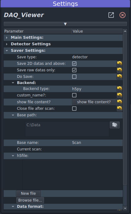
Fig. 2.23 Continuous Saving options

The saved file will follow this general structure:

D:\Data\2018\20181220\Data_20181220_16_58_48.h5

With a base path (D:\Data in this case) followed by a subfolder year, a subfolder day and a filename formed from a base name followed by the date of the day and the time at which you started to log data. Fig. 2.24 displays the tree structure of such a file, with two nodes (prefixed as enlargeable, EnlData) and a navigation axis corresponding to the timestamps at the time of each snapshot taken once the continuous saving has been activated (ticking the Do Save checkbox)

Fig. 2.24 Continuous Saving options