2.5.1.1. Introduction
DAQ_Scan automates data acquisition: it moves one or more actuators through a set of values and saves the data from the selected detectors at each position, in hierarchical HDF5 files.
2.5.1.1.1. Typical workflow
Define or load an experiment in the Dashboard first (see the experiment manager).
In the Actuators and Detectors panels, pick the actuators and detectors for the next scan.
In the Scan Parameters panel, choose the scan type (1D, 2D, …) and its subtype, then set the start, stop and step values of each actuator.
Use the Probe detectors button to list the data available from the selected detectors in the Plotting Parameters (all are ticked), and untick what should not be plotted live. Nothing is listed or plotted until then.
In the General Settings panel (gear button of the toolbar), check what is saved, how and where.
Press Start to run the scan. Stop ends it (scan flow).
2.5.1.1.2. Good to know
A dataset is one saved file that can contain several scans, usually for one sample or subject.
Live plots combine the dimension of the data with the scan dimension. Keep the total at 2 or less, and use regions of interest (ROI) to reduce raw data to a plottable form.
Saved files can be explored with the H5Browser extension.
Metadata are saved for each dataset and then for each scan and can be later retrieved from the saved file (see Module Savers and Data Browsing: the H5Browser module).
2.5.1.2. Main Control Window
The main control window is comprised of various toolbars, a Scan Command panel to set all parameters and a Live Plots panel displaying live data taken during a scan.
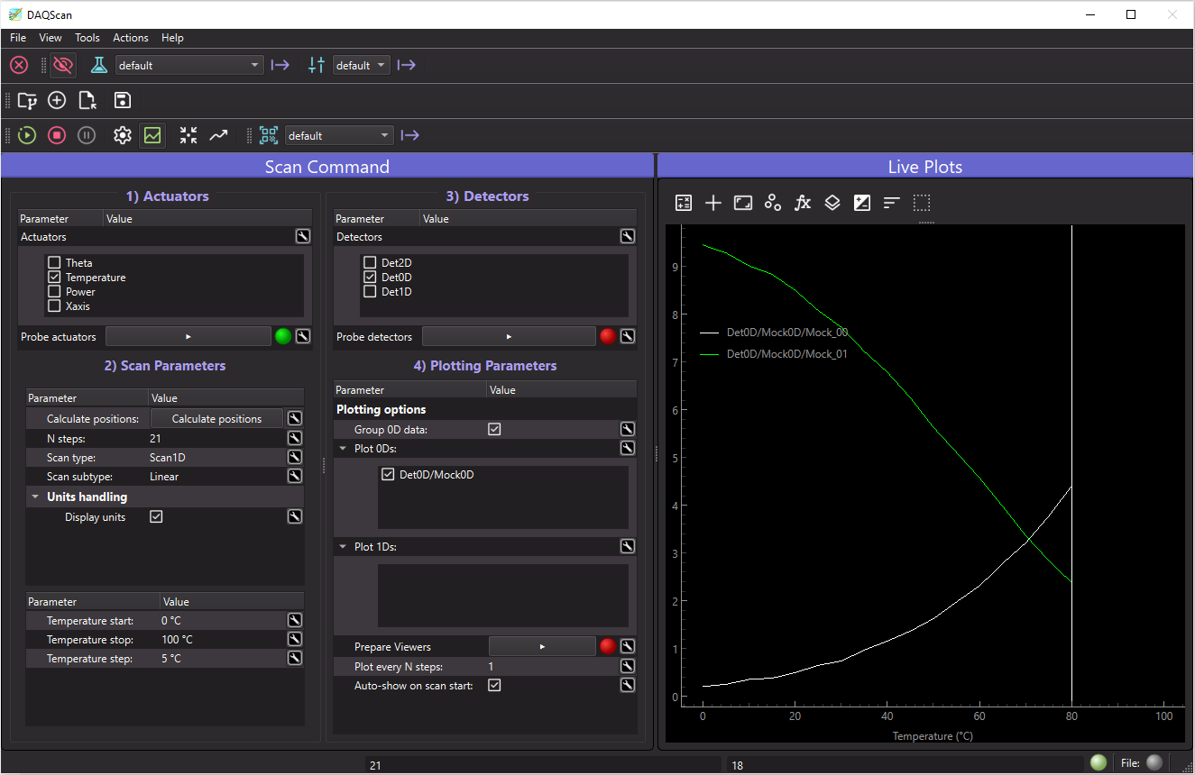
Fig. 2.34 Main DAQ_Scan user interface during a 1D scan. Left: the Scan Command panel with the Actuators and Detectors selection (top), the Scan Parameters and the Plotting Parameters (bottom). Right: the Live Plots panel.
The toolbars (top) allow to start, stop and pause a scan and to show or hide some panels, see Toolbar
The Actuators and Detectors panels allow to quickly select the actuators and the detectors to use for the next scan, and to probe them
The Scan Parameters panel allows to select the type of scan and to set its values
The Plotting Parameters panel allows to select which data produced from the selected detectors should be rendered live
The Live Plots panel renders the data as a function of the varying parameters, as selected in the Plotting Parameters. It is shown automatically when a scan starts (see Auto-show on scan start below) and can be hidden or detached from the window (double-click on its title bar).
The General Settings panel (hidden by default, see Settings for more details) gathers the options on timing, scan averaging, saving and the saver worker.
2.5.1.3. Scan Flow
2.5.1.3.1. Selecting detectors and actuators
The Actuators and Detectors panels are the user interface of the module manager (see Module Manager for
details). They list the actuators and the detectors declared in the experiment loaded in the Dashboard and allow the
user to select the ones for the next scan by ticking them (see Fig. 2.35). The Probe actuators and
Probe detectors buttons read the current positions of the selected actuators and do a snap of the selected
detectors: the results are listed in the Probed actuator positions and Probed detector data sections below. The LED
turns green when the probe is done. This interface is also used for the DAQ_Logger extension.
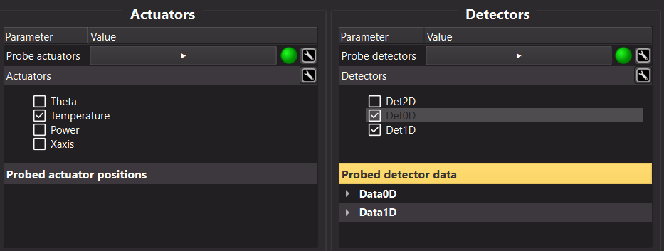
Fig. 2.35 The Actuators and Detectors panels: one actuator and two detectors are selected and have been probed.
2.5.1.3.2. Selecting the type of scan
All specifics of the upcoming scan are configured in the Scan Parameters panel, using the Scanner module interface, as seen on Fig. 2.36 in the case of a Scan2D scan configuration. Once the actuators are selected, choose the scan type (1D, 2D, …), its subtype (linear, random, spiral, …) and set the start, stop and step values of each actuator.
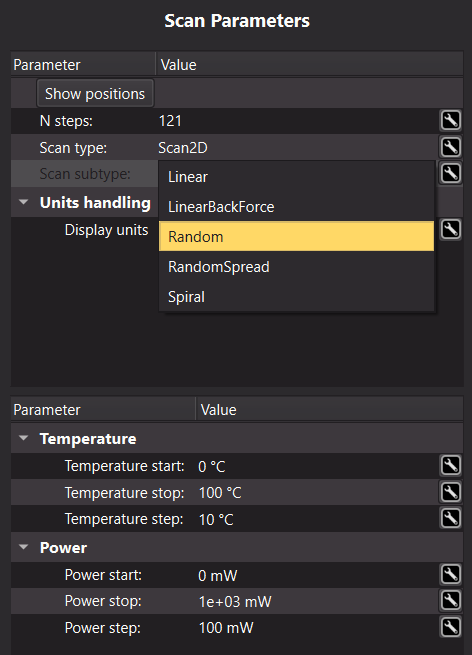
Fig. 2.36 The Scan Parameters panel set on a Scan2D scan type with two actuators (Temperature and Power), 121 steps in total. The list of the available scan subtypes (Linear, LinearBackForce, Random, RandomSpread, Spiral) is open; the start, stop and step values of each actuator are set in the lower table.
2.5.1.3.3. Selecting the data to render live
For a data acquisition system to be efficient, live data must be plotted in order to follow the experiment behaviour and check if something is going wrong or successfully without the need to perform a full data analysis. For this PyMoDAQ live data display will allows the user to select data to be plotted from the selected detectors.
The list of all possible data to be plotted is obtained by clicking on the Probe detectors button: the selected detectors are probed (a snap is done) and all the data they generate are listed in the Probed detector data section and in the Plotting options of the Plotting Parameters panel, classified by dimensionality (0D, 1D). They are all ticked by default: untick what should not be plotted. The total dimensionality of the data + the scan dimensions (1 for scan1D and 2 for Scan2D…) should not exceed 2 (this means one cannot plot more complex plots than 2D intensity plots). It also means that you should use ROI to generate lower dimensionality data from your raw data for a proper live plot.
For instance, if the chosen detector is a 1D one, see Fig. 2.37. Such a detector can generate various type of live data.
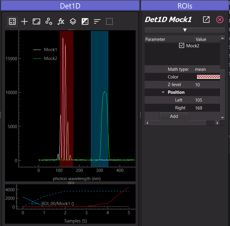
Fig. 2.37 An example of a 1D detector having 2 channels, with two regions of interest (set from the ROIs panel on the right, one on each channel). The bottom panel plots the history of their mean value (0D data).
It will export the raw 1D data and the 1D lineouts and integrated 0D data from the declared ROI as shown on Fig. 2.38
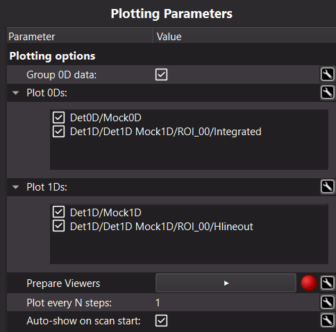
Fig. 2.38 The Plotting Parameters after probing a 0D and a 1D detector having an ROI (ROI_00). The 0D data (Plot 0Ds) are the one of the 0D detector and the integration of the ROI of the 1D detector. The 1D data (Plot 1Ds) are the raw data of the 1D detector and the lineout of its ROI.
Once the data to plot are selected, click on Prepare Viewers to generate the live plot panels (this is also done when starting a scan). One live plot panel will be created by selected data to be rendered with some specificities. One of these is that by default, all 0D data will be grouped on a single viewer panel, as shown on Fig. 2.34 (this can be changed using the Group 0D data option). Two more options control the live plots: Plot every N steps sets how often they are refreshed (1 for each scan point, 0 to disable live plotting during the scan) and Auto-show on scan start shows the Live Plots panel automatically when a scan starts.
The viewer type will be chosen (Viewer1D or 2D) given the dimensionality of the data to be ploted and the number of selected actuators.
if the scan is 1D:
exported 0D datas will be displayed on a
Viewer1Dpanel as a line as a function of the actuator position, see Fig. 2.34.exported 1D datas will be displayed on a
Viewer2Dpanel as color levels as a function of the actuator position, see Fig. 2.39.

Fig. 2.39 An example of a detector exporting 1D live data plotted as a function of the actuator position (here a Temperature scan in progress). The two channels of the 1D detector are plotted in red and green, the vertical white rectangle shows the position reached by the scan.
if the scan is 2D:
exported 0D datas will be displayed on a
Viewer2Dpanel as a pixel map where each pixel coordinates represents a scan coordinate. The color and intensity of the pixels refer to channels and data values, see Fig. 2.40 for a linear 2D scan.
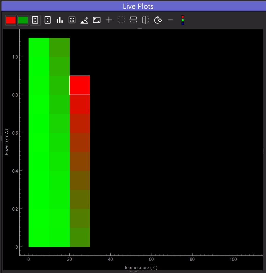
Fig. 2.40 An example of a detector exporting 0D live data (two channels, in red and green) plotted as a function of the 2 actuators’s position (Temperature and Power), scan in progress. The white rectangle is the last acquired point.
So at maximum, 2D dimensionality can be represented. In order to see live data from 2D detectors, one should therefore export lineouts from ROIs or integrate data. All these operations are extremely simple to perform using the ROI features of the data viewers (see Data viewers)
2.5.1.4. Various settings
2.5.1.4.1. Toolbar
The scan toolbar (see Fig. 2.41) is comprised of buttons to start, pause and stop a scan, to show or hide panels and to move the actuators:

Fig. 2.41 The scan toolbar while a scan is running (Start is disabled). From left to right: Start, Stop, Pause, Show General Settings, Show Live Plots, Init. Positions and Move at double clicked.
Start: will start the currently set scan (first it will set it then start it)
Stop: stop the currently running scan
Pause: toggle pause/resume on a running scan. The scan loop will wait until unpaused or stopped.
Show General Settings: show or hide the General Settings panel, see General Settings
Show Live Plots: show or hide the Live Plots panel
Init. Positions: will move all selected actuators to their initial positions as defined by the currently set scan.
Move at double clicked: when checked, allows currently selected actuators to be moved by double clicking on a position in the live plots
The top toolbar, shared with the Dashboard, allows to quit the application (red cross: it will shut down all modules, redundant with the File/Quit menu), to show the Dashboard and to load an experiment or a state. The Actions menu duplicates the actions of the scan toolbar.
2.5.1.4.2. Menu Bar Description
The menu bar has five entries: File, View, Tools, Actions and Help.
The File entry will let you:
Show the content of the current file in the H5Browser (Show file content)
Create a new file (New file)
Load a previously saved scan file and keep saving scans on it (Open file to append…)
Save a copy of the current file in another filename than the default one (Save copy as…)
Show the settings of the h5 file saver (Show h5 settings)
Restart or quit the application (Restart, Quit: the latter shuts down all modules)
The View entry will let you show or hide each of the toolbars (Toolbars) and change their style.
The Tools entry will let you:
show the Scan Manager toolbar, to save and reload complete scans (selected modules, scanner and scan parameters) as
.scanfiles, see Scan Managerdisplay the Navigator (see Navigator)
open the log file (Logs) and the PyMoDAQ Preferences
use the tools shared by all the PyMoDAQ applications: enable the scripting, run a LECO coordinator or start the Plugin Manager
The Actions entry gathers the actions of the extension, see Fig. 2.42. It starts with the
workflow actions common to the extensions (Start Workflow, Stop Workflow and Pause Workflow, that are the Start,
Stop and Pause buttons of the toolbar), followed by the actions specific to the extension: for the DAQ_Scan
Show General Settings, Show Live Plots, Init Positions and Move at doubleClicked, see Toolbar.
Most of the extensions put their own actions in this menu.
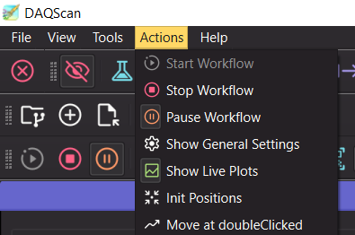
Fig. 2.42 The Actions menu of the DAQ_Scan.
The Help entry gives access to the online documentation (F1), to the check for new PyMoDAQ versions and to the
About window.
2.5.1.4.3. Status Bar
The status bar at the bottom of the window shows:
A message label with the current file name and scan name
Scan step counters (total steps and current step)
A Scan done LED indicator
A File LED indicator (green when the h5 file is open)
An SWMR label that shows:
SWMR when SWMR mode is actively in use during a scan
SWMR file when the opened file was created with SWMR support but SWMR is not currently active
hidden when the file has no SWMR association
2.5.1.4.4. Settings
The settings tree as shown on Fig. 2.34 is actually divided in a few subtrees that contain everything needed to define a given scan, save data and plot live information.
2.5.1.4.4.1. General Settings
The General Settings panel (see Fig. 2.43) is hidden by default. It is shown or hidden with the
Show General Settings button of the toolbar (or of the Actions menu), and double-clicking on its title bar detaches
it into its own window. To have it shown when the DAQ_Scan starts, set show_general_settings = true in the [scan]
section of the pymodaq configuration file (see Preferences files).

Fig. 2.43 The General Settings panel of the DAQ_Scan.
It is comprised of:
Time Flow
Wait time step: extra time the application wait before moving on to the next scan step. Enable rough timing if needed
Wait time between: extra time the application wait before starting a detector’s grab after the actuators reached their final value.
Scan options :
N average: Select how many scans to average. Save all individual scans. Averaging is not available for the scans generating spread data (Tabular and Scan2D/RandomSpread): N average is then set to 1 and locked.
Plot on top: at the second iteration, plot the averaged scan on top of the current one (checked) or in a second panel
Go to ini. positions: when checked (default), actuators are moved back to their initial positions when the scan ends or is stopped.
Stop on timeout: if a hardware timeout occurs while waiting for an actuator or a detector, stop the scan. If unchecked, the scan moves on to the next step.
Save: everything about what is saved, how and where, see Saving: Dataset and scans and H5Saver.
Saver Worker: status of the thread saving the data during the scan (running LED and number of pending save tasks)
The plotting options (Plot 0Ds, Plot 1Ds, Prepare Viewers…) are in the Plotting Parameters panel, see Selecting the type of scan.
2.5.1.4.4.2. Saving: Dataset and scans
DAQ_Scan module will save your data in datasets. Each dataset is a unique h5 file and may contain multiple scans. The idea behind this is to have a unique file for a set of related data (the dataset) together with all the meta information: logger data, module parameters (settings, ROI…) even png screenshots of the various panels.
Fig. 2.44 displays the content of a typical dataset file containing various scans and how each data and metadata is used by the Data Browsing: the H5Browser module to display the info to the user.

Fig. 2.44 h5 browser and arrows to explain how each data or metadata is being displayed
The Save settings, in the lower part of the General Settings panel (see Fig. 2.45), are the user interface of the H5Saver, a general interface to parametrize data saving in the hdf5 file. As the General Settings are hidden by default, use the Show General Settings button of the toolbar to display them:
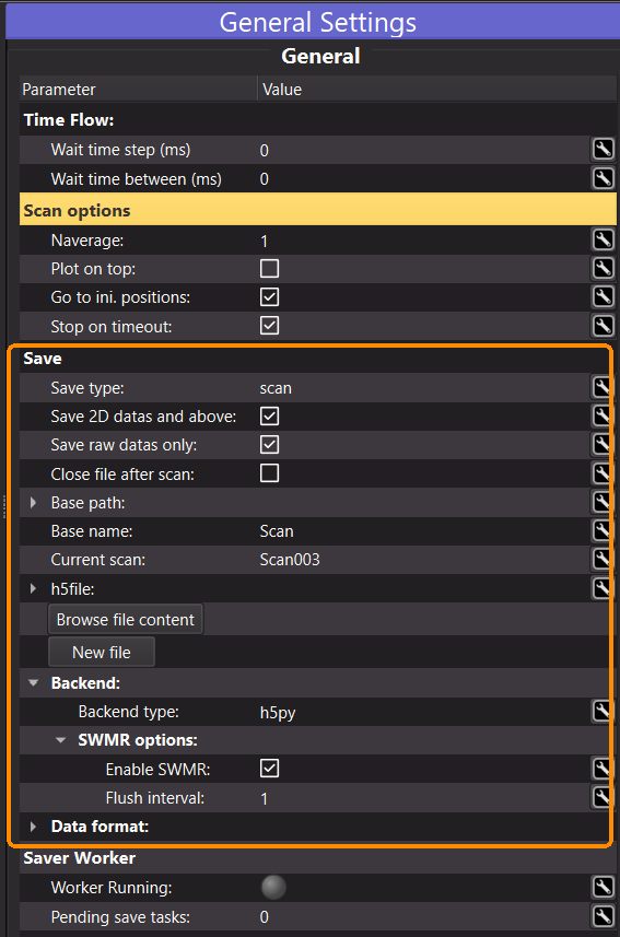
Fig. 2.45 The Save settings (orange rectangle) of the DAQ_Scan, in the lower part of the General Settings panel.