3.6.3. Simulating a spectro-photometer

In this section we will write the code for controlling a spectro-photometer. Let us begin with a brief comment on simulating devices. Simulating things is a useful starting point in this tutorial because we avoid communication issues with real devices for now. On top of that, no hardware is needed and the development can take place anywhere where an internet connection is available (the latter for installing missing stuff and searching for help when it doesn’t-doesn’t). However, it can be very useful to keep simulation capabilities in place even when everything works fine with real hardware.

There might be only a single and expensive device around and your colleagues are using it at present for a longer measurement campaign. With a simulated device you may happily continue coding.
Suppose that the experiment has a surprising result. Being able not only to simulate some default values but the outcome of an entire experiment while using the whole chain from the simulated device over PyMoDAQ’s functionality to data treatment software may be a very helpful quality control. Is the result surprising because a mistake happened during the experiment? during data acquisition? during treatment? or did we actually discover something new??
You may learn a lot about your experiment and its instrumentation by making sure that at the tail of the chain you are actually getting back exactly what you have put into the simulation at its head. Remember that the only way a sample can talk to you in a spectroscopic experiment is by means of signal photons it emits. These and the carried information pass by a multitude of optical elements, detectors, ADC converters, data treatment of all sorts etc. Quite some Chinese whispers to master.

To understand the spectroscopic peculiarities behind the code in this section, one has to dive into the detection of visible light to quite some extent. For those who don’t want to spend time on these details, you may just skip this section until here, where the checked-out code should readily reproduce the figures shown below. Just keep in mind as an advice, once you’ve got together a draft code of the experiment you want to control, it is probably still a good idea to simulate that experiment, instead of the one presented here where the details don’t matter to you.

We start with a controller situated in the hardware directory of the plugin (src/pymodaq_plugins_tutorial_extensions/hardware). When using real hardware, an instance of the controller is managing the communication with the device. In the absence of real hardware that wouldn’t be necessary. Nevertheless, we use the same structure here because a couple of simulated instruments will have to work together, sharing common “knowledge” about the state of the simulated experiment. And that will happen in the controller which is going to be shared by all plugins to be written. We use here a dataclass to avoid quite some boiler plate code at initialisation. Create a file controller.py in the hardware directory and fill in the following code

import time
import numpy as np
from dataclasses import dataclass


@dataclass
class MockSpectrograph:

    integration_time: float = 50
    n_pixels: int = 1024
    readout_noise: int = 4
    dark_level: float = 150
    light_level: float = 500
    pe_per_lsb: float = 18.3
    adc_bits: int = 16
    wl_from: float = 300
    wl_to: float = 900
    absorption: float = 0.3

    def __post_init__(self):
        self.calculate_base_data()

    def calculate_base_data(self):
        n_pix = self.n_pixels
        self.wavelengths = \
            np.linspace(self.wl_from, self.wl_to, n_pix)
        self.pixels = np.linspace(0, n_pix - 1, n_pix)
        self.spectrum = \
            np.exp(-((self.pixels - n_pix / 2) / (n_pix / 3))**4)
        self.absorption = \
            self.absorption \
            * np.exp(-((self.pixels - n_pix / 4) / (n_pix / 8))**2)

The method __post_init__ is called from within the dataclass’ __init__ method. calculate_base_data initialises the part of the simulation which does not change with the state of the experiment. It should be called each time one of the parameters used in there has changed.

To test whether this works correctly we add some code at the end of the file which will be executed only when the file is directly called in a Python interpreter. It uses matplotlib to visualise the calculated data.

...

if __name__ == '__main__':
    import matplotlib.pyplot as plt
    spectrograph = MockSpectrograph()

    plt.plot(spectrograph.wavelengths, spectrograph.spectrum)
    plt.plot(spectrograph.wavelengths, spectrograph.absorption)
    plt.legend(['light spectrum', 'absorption'])
    plt.show()

The result should look like

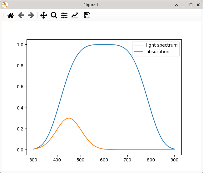
Of course, you’ll need to install matplotlib to make that working. At this point we have the first snippet of code running. You may checkout the branch

-> branch spectra

from the github repository to compare with your code, in case something doesn’t work as expected. You’ll find such a branch mark at each milestone of the tutorial, where code should be ready to run.

Next comes the method which is used to generate realistic spectroscopic data. Without light exposure detectors show some dark signal which is mostly coming from thermal noise. Its amplitude is typically proportional to the integration time. It comes in units of LSB (least significant bit), i.e. in increments of the ADC. In case the signal gets too strong, the ADC signal saturates at the highest possible value (e.g. 65535 for a 16 bit ADC). The simulated signal is therefore cut to that level. Together with the data we send a time stamp.

class MockSpectrograph:
    ...
    def simulate_spectrum(self, shutter_open: bool, sample: bool):
        data = np.random.normal(loc=self.dark_level * self.integration_time,
                                scale=self.readout_noise, size=self.n_pixels)

        max_adc = (1 << self.adc_bits) - 1
        data = np.where(data < max_adc, np.floor(data), max_adc)
        return data, time.time()

 if __name__ == '__main__':
     ...
     plt.show()

     dark, time_stamp = \
     spectrograph.simulate_spectrum(shutter_open=False, sample=False)
     plt.plot(dark)
     plt.title('dark')
     plt.show()

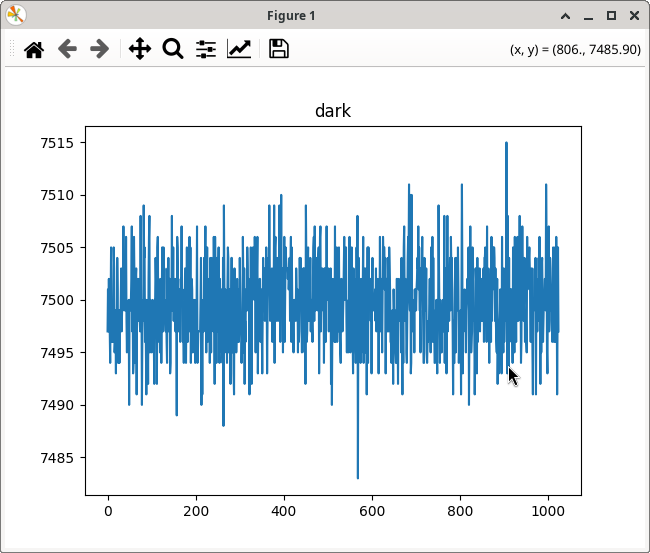
Note that we make simulate_spectrum returning two items, the required data and the time the function returns. Strictly speaking, this wouldn’t be necessary because PyMoDAQ also adds a time stamp to any data item. However, later on this can be used to demonstrate inspecting data by dimension or name or other.

-> branch background

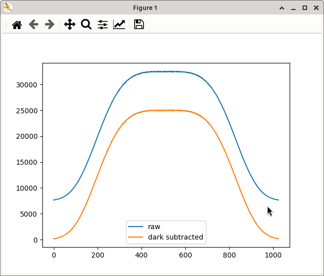
Once the probe light passes through the sample cell, but filled only with solvent, the light induces a photo current in the detector which is accumulated as charges in a capacitor during the integration time. The natural unit of the detected quantity would therefore be the number of collected photo electrons. However, the read-out is performed by discharging the capacitor through a resistance and measuring the voltage across this resistance by means of an ADC. Therefore, the property light_level is given in units of ADC LSB–because that is what the user sees on the plot showing the camera read-out–with the conversion factor pe_per_lsb (photo electrons per LSB).

The detected signal exhibits a fluctuation due to counting statistics. Other types of fluctuations like a variation of the overall amplitude due to correlated thermal noise could be implemented here as well. For the purpose of demonstration we’ll leave it at the level of counting statistics. Keep in mind that these counting statistics are based on the number of photo electrons collected per pixel. Before determining the spread of the corresponding Poisson distribution, the signal amplitude has to be converted into that number. And once the random numbers have been generated, they have to be converted back to ADC LSB.

 def simulate_spectrum(self, shutter_open: bool, sample: bool):
     data = np.random.normal(loc=self.dark_level * self.integration_time,
                             scale=self.readout_noise, size=self.n_pixels)
     if shutter_open:
         light = self.spectrum * self.light_level * self.integration_time \
             * self.pe_per_lsb
         data += np.random.poisson(light) / self.pe_per_lsb
     max_adc = (1 << self.adc_bits) - 1
     data = np.where(data < max_adc, np.floor(data), max_adc)

     return data, time.time()

 ...

     data, time_stamp = \
         spectrograph.simulate_spectrum(shutter_open=True, sample=False)
     plt.plot(data)
     reference = data - dark
     plt.plot(reference)
     plt.legend(['raw', 'dark subtracted'])
     plt.show()

-> branch signal-and-background

After having inserted an absorbing sample, the intensity of the light transmitted through the sample is reduced according to

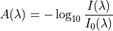
$A(\lambda) = -\log_{10}\frac{I(\lambda)}{I_0(\lambda)}$

where $A(\lambda)$ is the absorption measured as optical density, $I(\lambda)$ is the light transmitted through the sample and $I_0(\lambda)$ the intensity of the light transmitted through pure solvent.

 def simulate_spectrum(self, shutter_open: bool, sample: bool):
     data = np.random.normal(loc=self.dark_level * self.integration_time,
                             scale=self.readout_noise, size=self.n_pixels)
     if shutter_open:
         light = self.spectrum * self.light_level * self.integration_time \
             * self.pe_per_lsb
         if sample:
             light *= np.pow(10, -self.absorption)
         data += np.random.poisson(light) / self.pe_per_lsb
     max_adc = 1 << self.adc_bits
     data = np.where(data < max_adc, np.floor(data), max_adc)

     return data, time.time()

 ...

     data, time_stamp = \
         spectrograph.simulate_spectrum(shutter_open=True, sample=True)
     plt.plot(data)
     signal = data - dark
     plt.plot(data - dark)
     plt.legend(['raw through sample', 'dark subtracted'])
     plt.show()

The resulting spectra should look like follows

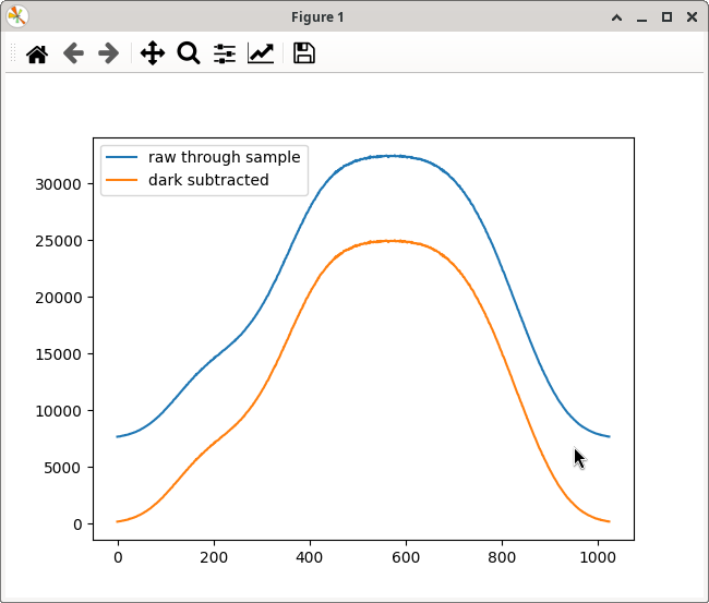
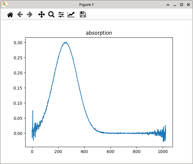
And finally, calculating the absorption from these data, the result should look like

plt.plot(-np.log10(signal / reference))
plt.title('absorption')
plt.show()

-> branch controller-ready