5.7. Tutorial On Data Manipulation and analysis
Author email |
|
Last update |
february 2024 |
Difficulty |
Intermediate |
This tutorial is directly extracted from a jupyter notebook used to illustrate how to get your data back from a PyMoDAQ h5 file, analyze it and plot interactively these data. You’ll find the notebook here.
This example is using experimental data collected on a time-resolved optical spectroscopy set-up developed by Arnaud Arbouet and “PyMoDAQed” by Sebastien Weber in CEMES.
Practical work sessions exploiting this set-up and data analysis are organized every year in the framework of the Master PFIQMC at University Toulouse III PauL Sabatier. The students have to align an ultrafast transient absorption experiment and acquire data from a gold thin film. In these pump-probe experiments, two femtosecond collinear light pulses are focused on the sample (see Fig. 5.73). The absorption by a first “pump” pulse places the sample out-of equilibrium. A second, delayed “probe” light pulse is used to measure the transmission of the sample during its relaxation.
The measured dynamics shows (i) the transmission change associated with the injection of energy by the pump pulse (< ps timescale) followed by (ii) the quick thermalization of the electron gas with the gold film phonons (ps timescale) and (iii) the oscillations induced by the mechanical vibrations of the film (10s ps timescale). To be able to detect these oscillations, one needs to repeat the pump-probe scan many times and average the data.
PyMoDAQ allows this using the DAQ_Scan extension. One can specify how many scan should be performed and both the current scan and the averaged one are displayed live. However all the individual scans are saved as a multi-dimensional array. Moreover, because of the different time-scales (for electrons and for phonons) a “Sparse” 1D scan is used. It allows to quickly specify actuator values to be scanned in pieces (in the form of multiple start:step:stop). For instance scanning the electronic time window using a low step value and the phonon time window with a higher time step. The scan is therefore perfectly sampled but the time needed for one scan is reduced.
The author thanks Dr Arnaud Arbouet for the data and explanations. And if you don’t understand (or don’t care about) the physics, it’s not an issue as this notebook is here to show you how to load, manipulate and easily plot your data.
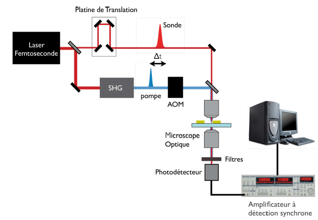
Fig. 5.73 Experimental Setup for time-resolved optical spectroscopy
To execute this tutorial properly, you’ll need PyMoDAQ >= 4.0.2 (if not released yet, you can get it from github)
%gui qt5
# magic keyword only used to start a qt event loop within the jupyter notebook framwork

# importing built in modules
from pathlib import Path
import sys

# importing third party modules
import scipy as sc
import scipy.optimize as opt
import scipy.constants as cst
import numpy as np

# importing PymoDAQ modules
from pymodaq.utils.h5modules.saving import H5SaverLowLevel  # object to open the h5 file
from pymodaq.utils.h5modules.data_saving import DataLoader  # object used to properly load data from the h5 file
from pymodaq.utils.data import DataRaw, DataToExport

from pymodaq import __version__
print(__version__)

LIGHT_SPEED = 3e8  #m/s
4.2.0
5.7.1. Loading Data
dwa_loader = DataLoader('Dataset_20240206_000.h5') # this way of loading data directly from a Path is
#available from pymodaq>=4.2.0

for node in dwa_loader.walk_nodes():
    if 'Scan012' in str(node):
        print(node)
/RawData/Scan012 (GROUP) 'DAQScan'
/RawData/Scan012/Actuator000 (GROUP) 'delay'
/RawData/Scan012/Detector000 (GROUP) 'Lockin'
/RawData/Scan012/NavAxes (GROUP) ''
/RawData/Scan012/Detector000/Data0D (GROUP) ''
/RawData/Scan012/NavAxes/Axis00 (CARRAY) 'delay'
/RawData/Scan012/NavAxes/Axis01 (CARRAY) 'Average'
/RawData/Scan012/Detector000/Data0D/CH00 (GROUP) 'MAG'
/RawData/Scan012/Detector000/Data0D/CH01 (GROUP) 'PHA'
/RawData/Scan012/Detector000/Data0D/CH00/Data00 (CARRAY) 'MAG'
/RawData/Scan012/Detector000/Data0D/CH01/Data00 (CARRAY) 'PHA'
To load a particular node, use the load_data method
dwa_loaded = dwa_loader.load_data('/RawData/Scan012/Detector000/Data0D/CH00/Data00')
print(dwa_loaded)
<DataWithAxes: MAG <len:1> (100, 392|)>
5.7.2. Plotting data
From PyMoDAQ 4.0.2 onwards, both the DataWithAxes (and its inheriting
children classes) and the DataToExport objects have a plot method.
One can specify as argument which backend to be used for plotting. At
least two are available: matplotlib and qt. See below
dwa_loaded.nav_indexes = ()  # this is converting both navigation axes: average and delay as signal axes (to be plotted in the Viewer2D)
dwa_loaded.plot('matplotlib')
or using PyMoDAQ’s data viewer (interactive and with ROIs and all other features)
dwa_loaded.plot('qt')
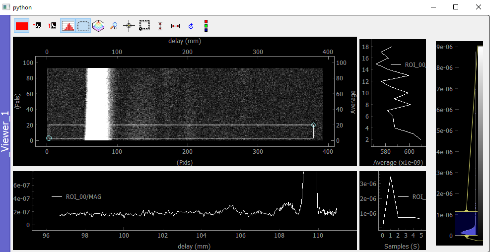
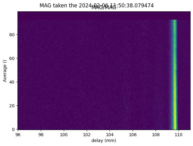
Fig. 5.74 python
The horizontal axis is a delay in millimeter (linear stage displacement, see setup) and we used a Sparsed scan with a non equal scan step (see figure below, right panel)
delay_axis = dwa_loaded.get_axis_from_index(1)[0]
dte = dwa_loaded.as_dte('mydata')
dte.append(DataRaw(delay_axis.label, data=[delay_axis.get_data()]))
dte.plot('qt')
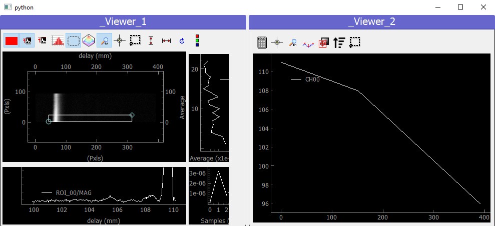
Fig. 5.75 python
dwa_loaded_steps = dwa_loaded.deepcopy()
delay_axis = dwa_loaded_steps.get_axis_from_index(1)[0]
delay_axis.data = delay_axis.create_simple_linear_data(len(delay_axis))
delay_axis.label = 'steps'
delay_axis.units = ''
This delay axis is for the moment in mm and reversed (the stage is going backwards to increase the delay). Let’s recreate a flipped axis with seconds as units.
dwa_loaded_fs = dwa_loaded.deepcopy()
delay_axis = dwa_loaded_fs.get_axis_from_index(1)[0]
delay_axis.data = - 2 * delay_axis.get_data() / 1000 / LIGHT_SPEED  # /1000 because the dsiplacement unit
# of the stage is in mm and the speed of light in m/s
delay_axis.data -= delay_axis.get_data()[0]
delay_axis.units = 's'
print(delay_axis.get_data()[0:10])
[0.00000000e+00 1.33333333e-13 2.66666667e-13 4.00000000e-13
 5.33333333e-13 6.66666667e-13 8.00000000e-13 9.33333333e-13
 1.06666667e-12 1.20000000e-12]
dwa_loaded_fs.plot('qt')
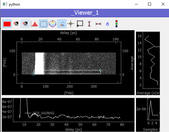
Fig. 5.76 python
5.7.3. Data Analysis
Now we got our data, one can extract infos from it
life-time of the electrons -> phonons thermalization
Oscillation period of the phonons vibration
To do this, one will properly slice the data correpsonding to the electrons and the one corresponding to the phonons. To get the scan index to use for slicing, one will plot the raw data as a function of scan steps and extract the index using ROIs
dwa_loaded_steps.plot('qt')
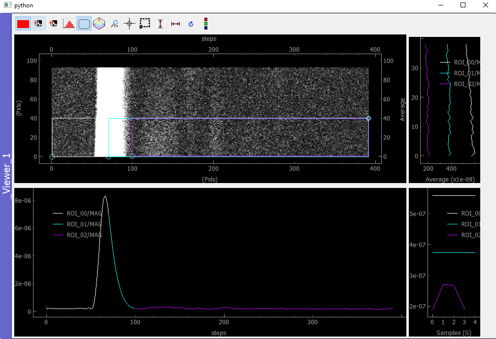
Fig. 5.77 python
5.7.3.1. Slicing the data
The ROi Manager (on the right, not visible here) tell us to use:
indexes_electrons = (70, 390)
indexes_phonons = (100, 300)
indexes_average = (0, 40) # we are not using all the averaging because the gold
# film seems to be dying as time goes on...
First we slice the data over the average indexes and the electron
indexes This is done easily using the isig slicer (sig for signal
axes. For navigation one should use the inav slicer). Those slicers return a DataWithAxes object
where data and axes have been sliced. Then we immediately apply the mean method over the average axis
(index 0) to get 1D dimensionality data:
dwa_electrons = dwa_loaded_fs.isig[slice(*indexes_average), slice(*indexes_electrons)].mean(0)
print(dwa_electrons)

dwa_phonons = dwa_loaded_fs.isig[slice(*indexes_average), slice(*indexes_phonons)].mean(0)
print(dwa_phonons)
<DataWithAxes: MAG <len:1> (|320)>
<DataWithAxes: MAG <len:1> (|200)>
dte = DataToExport('mydata', data=[dwa_electrons, dwa_phonons])
print(dte)
dte.plot('qt')
DataToExport: mydata <len:2>
    * <DataWithAxes: MAG <len:1> (|320)>
    * <DataWithAxes: MAG <len:1> (|200)>
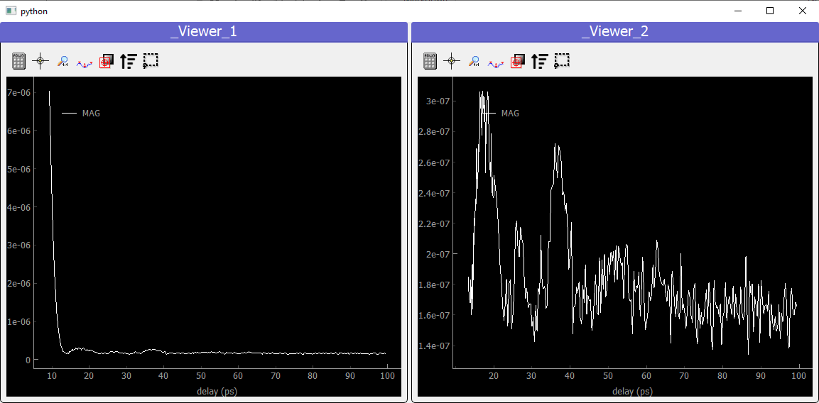
Fig. 5.78 python
5.7.3.2. Fitting the Data
5.7.3.2.1. Electrons:
def my_lifetime(x, A, B, C, tau):
    return A + C * np.exp(-(x - B)/tau)

time_axis = dwa_electrons.axes[0].get_data()
initial_guess = (2e-7, 10e-12, 7e-6, 3e-11)

dwa_electrons_fitted = dwa_electrons.fit(my_lifetime, initial_guess=initial_guess)
dwa_electrons_fitted.append(dwa_electrons)
dwa_electrons_fitted.plot('qt')
<pymodaq.utils.plotting.data_viewers.viewer1D.Viewer1D at 0x2ae0556cb80>
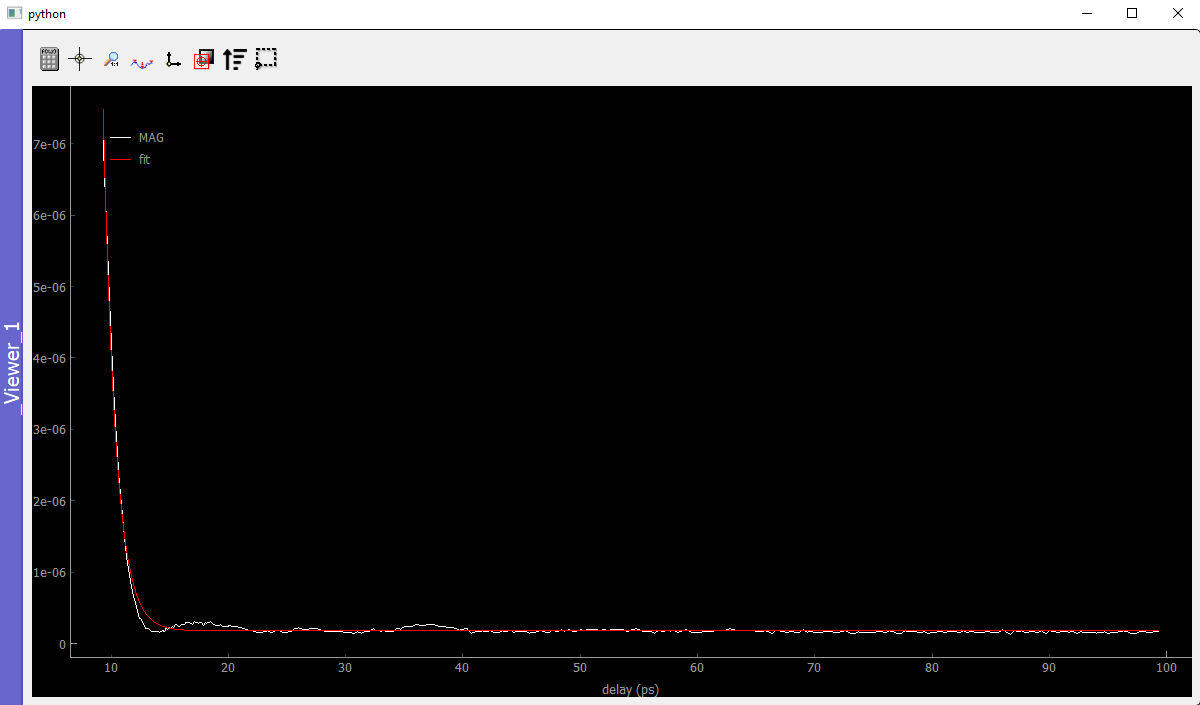
Fig. 5.79 python
One get a life time of about:
f'Life time: {dwa_electrons_fitted.fit_coeffs[0][3] *1e12} ps'
'Life time: 1.0688184683663233 ps'
5.7.3.2.2. Phonons:
For the phonons, it seems we have to analyse oscillations. The best for this is a Fourier Transform analysis. However because of the sparse scan the sampling at the begining is different from the one at the end. We’ll have to resample our data on a regular grid before doing Fourier Transform
5.7.3.2.2.1. Resampling
from pymodaq.utils import math_utils as mutils
from pymodaq.utils.data import Axis
phonon_axis_array = dwa_phonons.get_axis_from_index(0)[0].get_data()
phonon_axis_array -= phonon_axis_array[0]
time_step = phonon_axis_array[-1] - phonon_axis_array[-2]
time_array_linear = mutils.linspace_step(0, phonon_axis_array[-1], time_step)
dwa_phonons_interp = dwa_phonons.interp(time_array_linear)

dwa_phonons_interp.plot('qt')
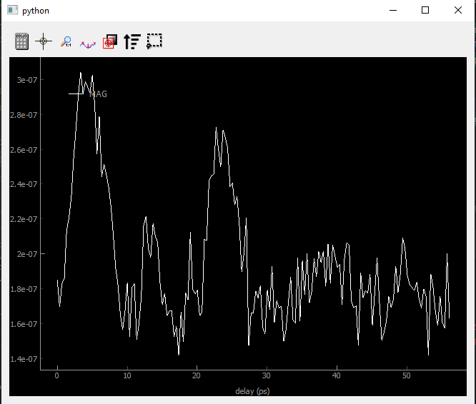
Fig. 5.80 Interpolated data on a regular time axis
5.7.3.2.2.2. FFT
dwa_fft = dwa_phonons_interp.ft()

dwa_phonons_fft = DataToExport('FFT', data=[
    dwa_phonons_interp,
    dwa_fft.abs(),
    dwa_fft.abs(),
    dwa_fft.abs()])
dwa_phonons_fft.plot('qt')
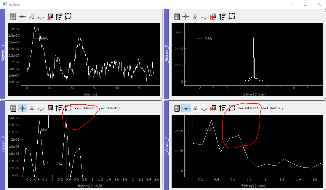
Fig. 5.81 Temporal data and FFT amplitude (top). Zoom over the two first harmonics (bottom)
Using advanced math processors to extract data from dwa:
from pymodaq.post_treatment.process_to_scalar import DataProcessorFactory
data_processors = DataProcessorFactory()
print('Implemented possible processing methods, can be applied to any data type and dimensionality')
print(data_processors.keys)
dwa_processed = data_processors.get('argmax').process(dwa_fft.abs())
print(dwa_processed[0])
Implemented possible processing methods, can be applied to any data type and dimensionality
['argmax', 'argmean', 'argmin', 'argstd', 'max', 'mean', 'min', 'std', 'sum']
[0.]
or using builtin math methods applicable only to 1D data:
dte_peaks = dwa_fft.abs().find_peaks(height=1e-6)
print(dte_peaks[0].axes[0].get_data() / (2*np.pi))

dte_peaks[0].axes[0].as_dwa().plot('matplotlib', 'o-r')  # transforms an Axis object to dwa for quick plotting

dte_peaks[0].get_data_as_dwa(0).plot('matplotlib', 'o-b')  # select part of the data object for "selected" plotting
[-1.06435192e+11 -5.32175961e+10  0.00000000e+00  5.32175961e+10
  1.06435192e+11]
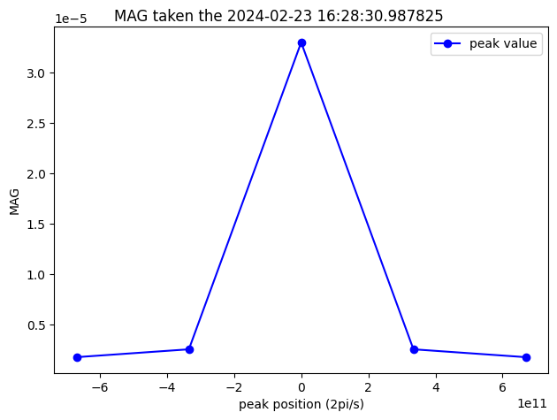
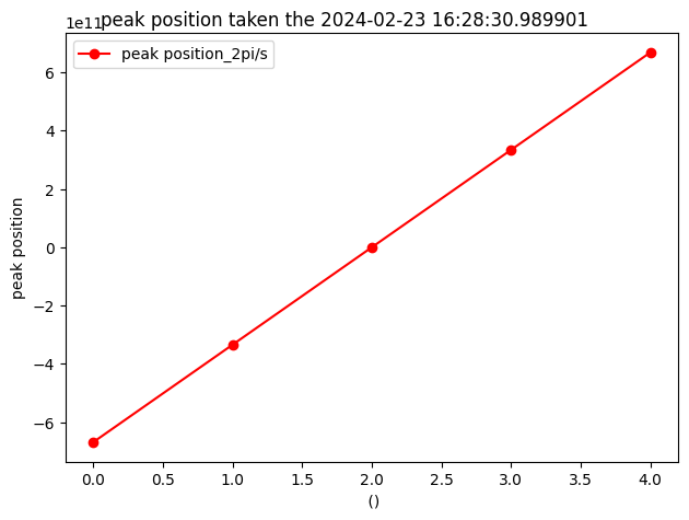
From this one get a fundamental frequency of 5.32e10 Hz that corresponds to a period of:
T_phonons = 1/5.32e10
print(f'Period T = {T_phonons * 1e12} ps')
Period T = 18.796992481203006 ps
From this period and the speed of sound in gold, one can infer the gold film thickness:
thickness = T_phonons / 2 * SOUND_SPEED_GOLD
print(f"Gold Thickness: {thickness * 1e9} nm")
Gold Thickness: 30.45112781954887 nm
5.7.4. Summary
To summarize this tutorial, we learned to:
easily load data using the DataLoader object and its load_data method (also using the convenience walk_nodes method to print all nodes from a file)
easily plot loaded data using the plot method (together with the adapted backend)
manipulate the data using its axes, navigation indexes, slicers and built in mathematical methods such as mean, ‘abs’, Fourier transforms, interpolation, fit…
For more details, see Data Management