5.4. Story of an instrument plugin development

In this tutorial, we will explain step by step the way to develop an instrument plugin. It is a specific type of plugin, that will allow you to control your device through PyMoDAQ.

As PyMoDAQ is not a library for professional developers, we consider that you reader do not know anything about how the development of an open source project works. We will take the time to start from scratch, and allow us to expand the scope of this documentation out of PyMoDAQ itself, to introduce Python environment, Git, external python libraries…

Rather than looking for a general and exhaustive documentation, we will illustrate the development flow with a precise example. We will go step by step through the development of the PI E-870 controller instrument plugin: from the reception of the device up to controlling it with PyMoDAQ. This one is chosen to be quite simple and standard. This controller can be used for example to control PiezoMike actuators, as illustrated below.

Fig. 5.9 The PI E-870 controller and PiezoMike actuators mounted on an optical mount.

The benefit of writing an instrument plugin is twofold:

• Firstly, you will learn a lot about coding, and coding the good way! Using the most efficient tools that are used by professional developpers. We will introduce how to use Python editors, linters, code-versioning, testing, publication, bug reporting, how to integrate open-source external libraries in your code… so that in the end you have a good understanding of how to develop a code in a collaborative way.

• Secondly, writing an instrument plugin is a great opportunity to dig into the understanding of your hardware: what are the physical principles that make my instrument working? How to fully benefit of all its functionalities? What are the different communication layers between my device and my Python script?

Writing an instrument plugin is very instructive, and perfectly matches a student project.

5.4.1. The controller manual

Let’s not be too impatient and take the time to read the controller manual, in the introduction we can read

“the E-870 is intended for open-loop operation of PIShift piezo inertia drives.” (page 3)

Ok but what is this PIShift thing? It is quite easy to find those videos that make you understand in a few tens of seconds the operating principle of the actuator:

PIShift drive principle

PiezoMike linear actuator

Nice! :)

What is open-loop operation? It means the system has no reading of the actuator position, as opposed to a close-loop operation. The open-loop operation is simpler and cheaper, because it does not require any encoder or limit switch, but it means that you will have no absolute reference of your axis, and less precision. This is an important choice when you buy an actuator, and it depends on your application. This will have big impact on our instrument plugin development.

“The E-870 supports one PIShift channel. The piezo voltage of the PIShift channel can be transferred to one of two (E-870.2G) or four (E-870.4G) demultiplexer channels, depending on the model. Up to two or four PIShift drives can be controlled serially in this manner.” (page 19)

Here we learn that in this controller, there is actually only one channel followed by a demultiplexer that will distribute the amplified current to the addressed axis. This means that only one axis can be moved at a time, the drives can only be controlled serially. This also depends on your hardware, and is an important information for the instrument plugin development.

5.4.2. The installer

It is important to notice that PyMoDAQ itself does not necessarily provide all the software needed to control your device. Most of the time, you have to install drivers, which are pieces of software, specific to each device, that are indispensable to establish the communication between your device and the operating system. Those are necessarily provided by the manufacturer. The ones you will install can depend on your operating system, and also on the way your establish the communication between them. Most of the time, you will install the USB driver for example, but this is probably useless if you communicate through Ethernet.

Let’s now run the installer provided in the CD that comes with the controller. The filename is PI_E-870.CD_Setup.exe. It is an executable file, which means that it hosts a program.

Fig. 5.10 The GUI of the installer.

On the capture on the right, you can see what it will install on your local computer, in particular:

• Documentation.

• A graphical user interface (GUI) to control the instrument, called the PI E870Control.

• Labview drivers: we will NOT need that! ;)

• A DLL library: PI GCS DLL. We will talk about that below.

• Some programming examples to illustrate how to communicate with the instrument depending on the programming language you use.

• USB drivers.

Whatever the way you want to communicate with your device, you will need the drivers. Thus, again, you need to install them before using PyMoDAQ.

Once those are installed, plug the controller with a USB cable, and go to the Device settings of Windows. An icon should appear like in the following figure. It is the first thing to check when you are not sure about the communication with your device. If this icon does not appear or there is a warning sign, change the cable or reinstall the drivers, no need to go further. You can also get some information about the driver.

Fig. 5.11 The Device settings window on Windows.

In the following, we will follow different routes, as illustrated in the following figure to progressively achieve the complete control of our actuator with PyMoDAQ. In the following we will name them after the color on the figure.

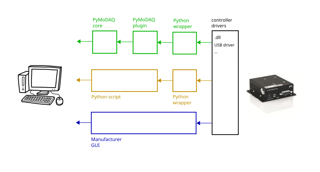
Fig. 5.12 The different routes (blue, gold, green) to establish the communication between the computer and the controller.

5.4.3. The blue route: use the manufacturer GUI

The simplest way to control your device is to use the GUI software that is provided by the manufacturer. It is usefull while you are under development, but will be useless once you have developped your plugin. PyMoDAQ will replace it, and even provide much broader functionalities. While a specific manufacturer GUI talks to only one specific device, PyMoDAQ provides to you a common framework to talk to many different instruments, synchronize them, save the acquisitions, and many more!

In the main tab, we found the buttons to send relative move orders, change the number of steps, change the controlled axis (in this example we can control 4 axis). Check all that works properly.

The second tab goes to a lower level. It allows us to directly send commands from the PI GCS library. We will see that below.

Fig. 5.13 Captures of the GUI provided by PI. Left: Interface to move the actuators and change the axis. Right: Interface to send GCS commands (see below).

Whenever you want to control a device with PyMoDAQ for the first time, even if you do not develop a plugin, you should first check that the manufacturer software is able to control your device. It is a prerequisite before using PyMoDAQ. By doing so we already checked a lot of things:

• The drivers are correctly installed.

• The communication with the controller is OK.

• The actuators are moving properly.

We are now ready for the serious part!

5.4.4. A shortcut through an existing green route? Readily available PyMoDAQ instrument plugins

Before dedicating hours of work to develop your own solution, we should check what has already been done. If we are lucky, some good fellow would already have developped the instrument plugin for our controller!

Here is the list of readily available plugins.

Each plugin is a Python package, and also a Git repository (we will talk about that later).

By convention, an instrument plugin can be used to control several devices, but only if they are from the same manufacturer. Those several hardwares can be actuators or detectors of different dimensionalities. The naming convention for an instrument plugin is

pymodaq-plugins-<manufacturer name>

Note

Notice the “s” at the end of “plugins”.

Note

Any kind of plugin should follow the naming convention pymodaq-plugins-<something more specific>, but an instrument plugin is a specific kind of plugin. For (an advanced) example, imagine that we create a beam pointing stabilization plugin, and that this system uses devices from different companies. We could have an actuator class that controls a SmarAct optical mount, a detector class that control a Thorlabs camera, and a PID model specifically designed for our needs. In that case we could use the name pymodaq-plugins-beam-stabilization.

All the plugins that are listed there can directly be installed with the plugin manager.

Some of those - let say the official ones - are hosted by the PyMoDAQ organization on GitHub, but they can also be hosted by other organizations. For example, the repository pymodaq-plugins-greateyes is hosted by the ATTOLab organization, but you can directly install it with the plugin manager.

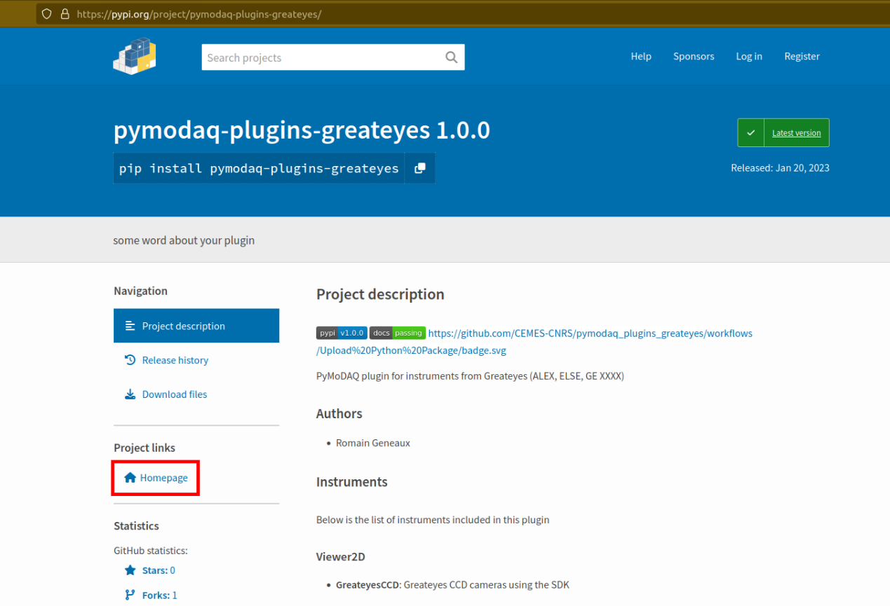
Fig. 5.14 The PyPI page of the greateyes plugin. If you click on Homepage you will find the Git repository page.

Remember that the already developed plugins will give you a lot of working examples, probably the way you will develop your own plugin will be very similar to one that already exist.

It sounds like we are very lucky… the PI plugin already exists!

Fig. 5.15 There is already a PI plugin in the list of available plugins.

Let’s try it!

Firstly, we have to install PyMoDAQ in a dedicated Python environment, that we will call pmd_dev in this tutorial.

Now that PyMoDAQ is installed and you have activated your environment (the lign of your terminal should start with (pmd_dev)), we will try to install the PI instrument plugin with the plugin manager. In your terminal, execute the following command

(pmd_dev) >plugin_manager

This will pop-up a window like this, select the plugin we are interested in and click Install

Fig. 5.16 Interface of the plugin manager.

Now let’s launch a DAQ_Move

(pmd_dev) >daq_move

Fig. 5.17 DAQ Move interface.

1. The list of available actuator contains the PI one, that sounds good!

2. Let select the USB connection type.

3. The list of available devices contains our controller with his serial number! That sounds really good because it means that the program can see the controller!

4. Let’s launch the initialization! Damn. The LED stays red! Something went wrong…

In a perfect world this should work, since we followed the proper way. But PyMoDAQ is a project under development, and some bugs may appear. Let’s not be discouraged! Actually we should be happy to have found this bug, otherwise we would not have the opportunity to explain how to face it.

What do we do now?

First, let’s try to get more information about this bug. PyMoDAQ automatically feeds a log file, let’s see what it has to tell us. You can find it on your computer at the location

<OS username>/.pymodaq/log/pymodaq.log

or you can open it through the Dashboard menu :

File > Show log file

It looks like this

Fig. 5.18 The log file of PyMoDAQ after trying to initialize the plugin.

This log file contains a lot of information that is written during the execution of PyMoDAQ. It is sorted in chronological order. If you find a bug, the first thing to do is thus to go at the end of this file.

In the above capture, we see that the first line indicates the moment we clicked on the Initialization button of the interface.

In the following we see that an error appeared: Unknown command (2). The least we can say is that it is not crystal clear to deduce the error from this!

At this point, we will not escape from digging into the code. If you do not feel like it, there is a last but very important thing that you can do, which is to report the bug. Try to detail as much as possible every step of your problem, and copy paste the part of the log file that is important. Even if you do not provide any solution, this reporting will be a usefull step to make PyMoDAQ better.

You dispose of several ways to do so.

1. Leave a message in the PyMoDAQ mailing list pymodaq@services.cnrs.fr.

2. Leave a message to the developper of the plugin.

3. Raise an issue on the GitHub repository associated to the plugin (you need to create an account, which is free). This last option is the most efficient because it targets precisely the code that raises a problem. Plus it will stay archived and visible to anyone that would face the same problem in the future.

Fig. 5.19 How to raise an issue on a GitHub repository.

Now we have gone as far as possible we could go without digging into the code, but if you are keen on it, let’s continue on the gold route (Fig. 5.12)!

5.4.5. The gold route: control your device with a Python script

We are now ready to tackle the core of this tutorial, and learn how to write a Python code to move our actuator. Let’s first introduce some important concepts.

5.4.5.1. What is a DLL?

As you may have noticed, the installer saved locally a file called PI_GCS2_DLL.dll.

The .dll file is a library that contains functions that are written in C++. It is an API between the controller and a computer application like PyMoDAQ or the PI GUI. It is made so that the person that intends to communicate with the controller is forced to do it the proper way (defined by the manufacturer’s developers). You cannot see the content of this file, but it is always provided with a documentation.

If you want to know more about DLLs, have a look at the Microsoft documentation.

Note

We suppose in this documentation that you use a Windows operating system, because it is the vast majority of the cases, but PyMoDAQ is also compatible with Linux operating systems. If you wish to control a device with a Linux system, you have to be careful during your purchase that your manufacturer provides Linux drivers, which is unfortunately not always the case. The equivalent of the .dll format for a Linux operating system is a .so file. PI provide such file, which is great! The development of Linux-compatible plugins will be the topic of another tutorial.

The whole thing of the gold route is to find how to talk to the DLL through Python.

In our example, PI developped a DLL library that is common to a lot of its controllers, called the GCS 2.0 library (it is the 2.0 version that is adapted to our controller). The associated documentation is quite impressive at first sight: 100+ (harsh!) pages.

This documentation is supposed to be exhaustive about all the functions that are provided by the library to communicate with a lot of controllers from PI. Fortunately, we will only need very few of them. The challenge here is to pick up the good information there. This is probably the most difficult part of an instrument plugin development. This is mostly due to the fact that there is no standardization of the way the library is written. Thus the route we will follow here will probably not be exactly the same for another device. Here we also depend a lot on the quality of the work of the developers of the library. If the documentation is shitty, that could be a nightmare.

Note

Our example deals with a C++ DLL, but there are other ways to communicate with a device: ASCII commands, .NET libraries (using pythonnet)…

5.4.5.2. What is a Python wrapper?

As we have said in the previous section, the DLL is written in C++. We thus have a problem because we talk the Python! A Python wrapper is a library that defines Python functions to call the DLL.

5.4.5.3. PIPython wrapper

Now that we introduced the concepts of DLL and Python wrapper, let’s continue with the same philosophy. We want to be efficient. We want to go straight to the point and code as little as possible. We are probably not the first ones to want to control our PI actuator with a Python script! Asking a search engine about “physik instrumente python”, we directly end up to the PI Python wrapper called PIPython.

Fig. 5.20 The PIPython repository on GitHub.

We can now understand a bit better the error given in the PyMoDAQ log earlier. It actually refers to the pipython package. This is because the PI plugin that we tested actually uses this library.

Note

All the Python packages of your environment are stored in the site-packages folder. In our case the complete path is C:\Users\<OS username>\Anaconda3\envs\pmd_dev\Lib\site-packages. Be careful to not end up in the base environment of Anaconda, which is located at C:\Users\<OS username>\Anaconda3\Lib\site-packages.

That’s great news! The PI developpers did a great job, and this will save us a lot of time. Unfortunately, this is not always the case. There are still some less serious suppliers that do not provide an open-source Python wrapper. You should consider this as a serious argument before you buy your lab equipment, as it can save you a lot of time and struggle. Doing so, you will put some pressure on the suppliers to develop Python open-source code, so that we can free our lab instruments!

5.4.5.4. External open-source libraries

In our example, our supplier is serious. Probably the wrapper it developped will do a good job. But let us imagine that it is not the case, and take a bit of time to present a few external libraries.

PyMoDAQ is of course not the only project of its kind. You can find on the internet a lot of non-official resources to help you communicate with your equipment. Some of them are so great and cover so much instruments that you should automatically check if your device is supported. Even if your supplier proposes a solution, it can be inspiring to have a look at them. Let’s present the most important ones.

PyLabLib

PyLabLib is a very impressive library that interfaces the most common instruments that you will find in a lab:

• Cameras: Andor, Basler, Thorlabs, PCO…

• Stages: Attocube, Newport, SmarAct…

• Sensors: Ophir, Pfeiffer, Leybold…

… but also lasers, scopes, Arduino… to cite a few!

Here is the complete list of supported instruments.

Here is the GitHub repository.

PyLabLib is extremely well documented and the drivers it provides are of extremely good quality: a reference!

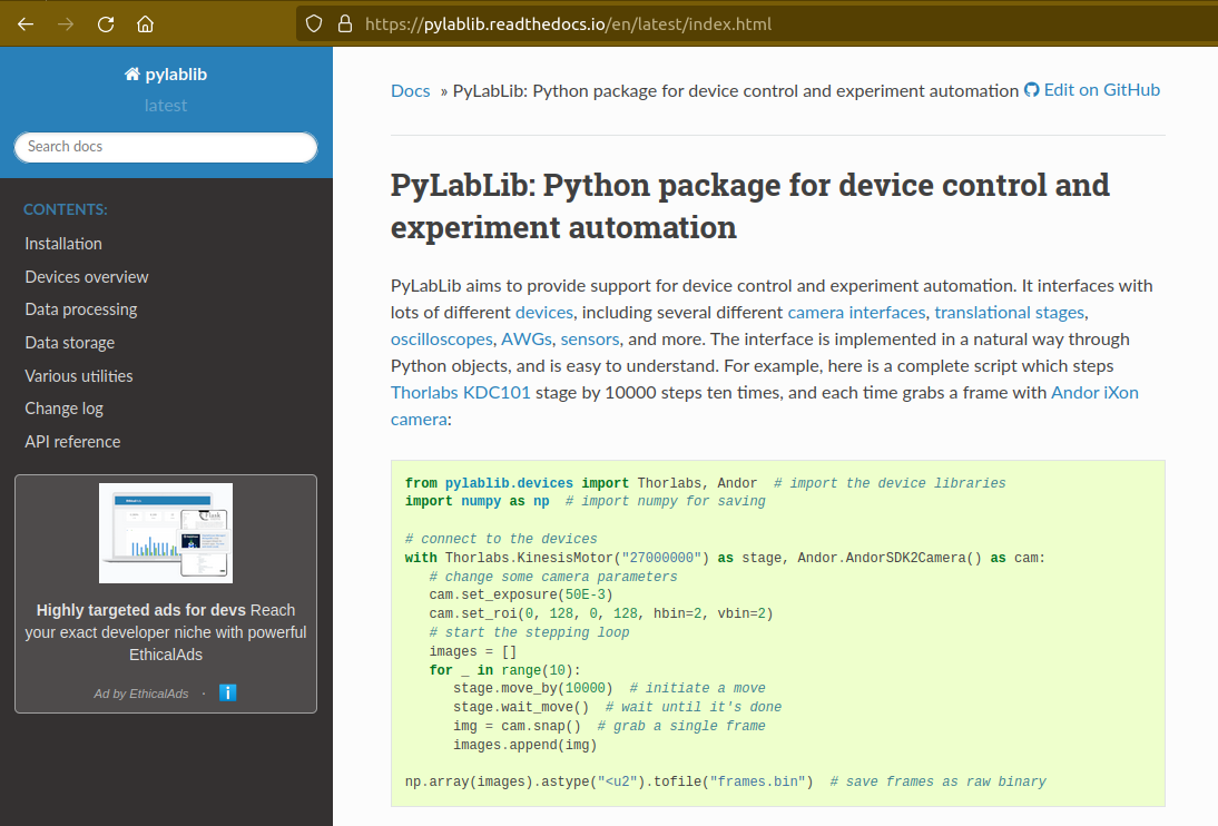
Fig. 5.21 The PyLabLib website.

Of particular interest are the camera drivers, that are often the most difficult ones to develop. It also proposes a GUI as a side project to control cameras: cam control.

Instrumental

Instrumental is also a very good library that you should know about, which covers different instruments.

Here is the list of supported instruments.

As you can see with the little script that is given as an example, it is super easy to use.

Instrumental is particularly good to create drivers from DLL written from C where one have the header file, autoprocessing the function signatures…

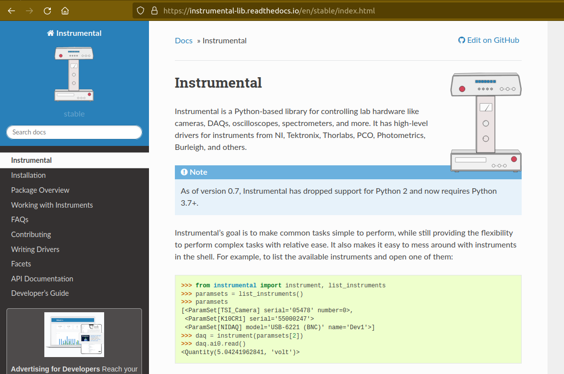
Fig. 5.22 The Instrumental website.

PyMeasure

PyMeasure will be our final example.

You can find here the list of supported instruments by the library.

This libray is very efficient for all instruments that communicate through ASCII commands (pyvisa basically) and makes drivers very easy to use and develop.

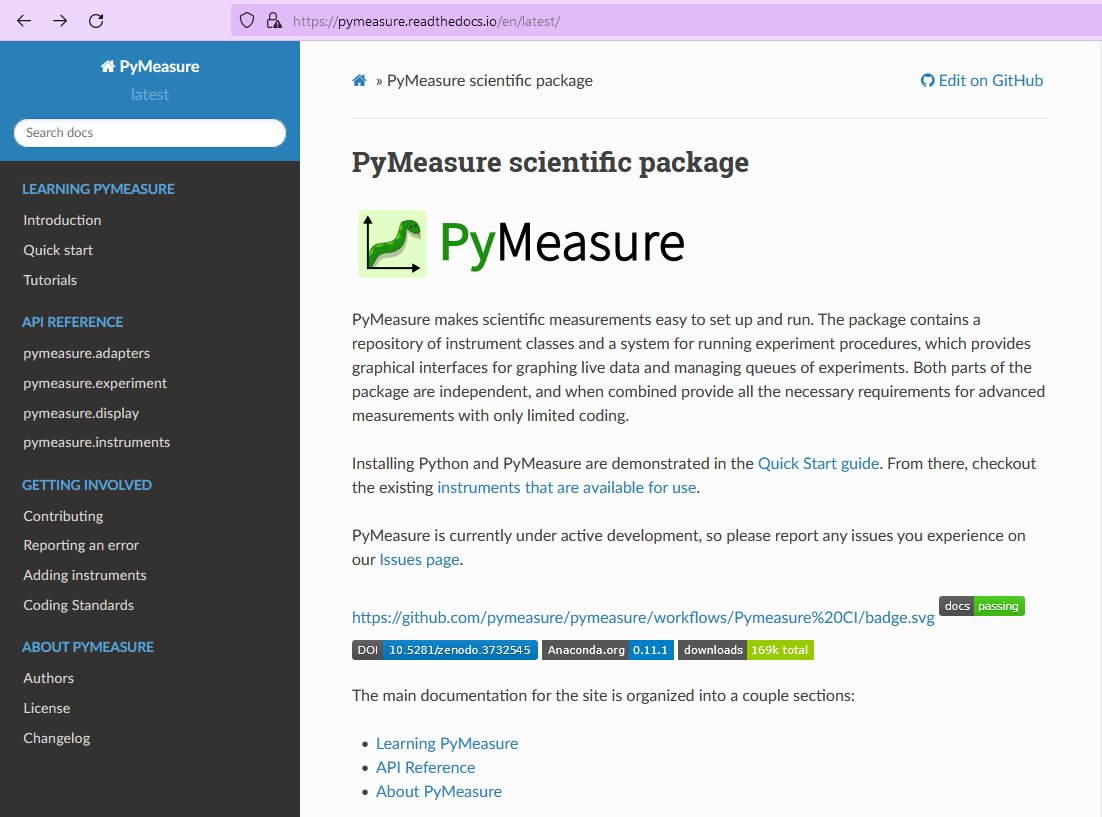
Fig. 5.23 The PyMeasure website.

Installation of external librairies

The installation of those libraries in our environment cannot be simpler:

(pmd_dev) >pip install <library name>

This list is of course not exhaustive. Those external ressources are precious, they will often provide a good solution to start with!

5.4.5.5. Back to PIPython wrapper

Let’s now go back to our E870 controller, it is time to test the PIPython wrapper!

We will install the package pipython in our pmd_dev environment

(pmd_dev) >pip install pipython

after the installation, we can check that the dependencies of this package have been installed properly using

(pmd_dev) >conda list

which will list all the packages that are installed in our environment

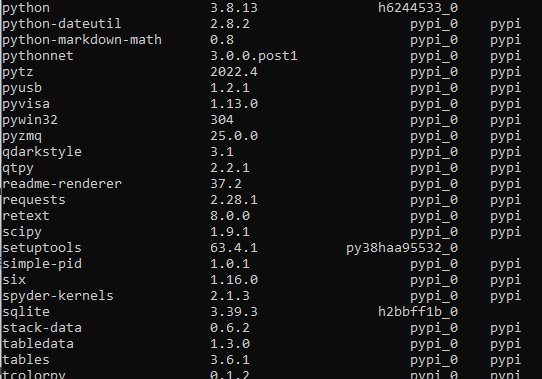
Fig. 5.24 List (partial) of the packages that are installed in our environment after installing pipython. We can check that the packages pyusb, pysocket and pyserial are there, as requested by the documentation.

Here we found the documentation of the wrapper.

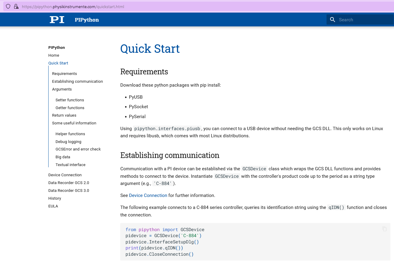
Fig. 5.25 Quick Start documentation of PIPython to establish the communication with a controller.

It proposes a very simple script to establish the communication. Let’s try that!

We will use the Spyder IDE to deal with such simple script, which is freely available. If you already installed an Anaconda distribution, it should already be installed.

Let’s open it and create a new file that we call script_pmd_pi_plugin.py and copy-paste the script.

It is important that you configure Spyder properly so that the import statement at the begining of the file will be done in our Python environment, where we installed the PIPython package. For this, click on the settings icon as indicated in the following capture.

Fig. 5.26 Running the PIPython quickstart script in the Spyder IDE.

The following window will appear. Go to the Python interpreter tab and select the Python interpreter (a python.exe file for Windows) which is at the root of your environment (in our case our environment is called pmd_dev. Notice that it is located in the envs subfolder of Anaconda). Do not forget to Apply the changes.

Fig. 5.27 Configure the good Python interpreter in Spyder.

Let’s now launch the script clicking the Run button. A pop-up window appears. We have to select our controller, which is uniquely identify by its serial number (SN). In our exemple it is the one that is underlined in blue in the capture. It seems like nothing much happens…

Fig. 5.28 Communication established!

…but actually, we just received an answer from our controller!

The script returns the reference and the serial number of our controller. Plus, we can see in the Variable explorer tab that the pidevice variable is now a Python object that represents the controller. For now nothing happens, but this means that our system is ready to receive orders. This is a big step!

Fig. 5.29 System ready.

Now, we have to understand how to play with this GCSDevice object, and then we will be able to play with our actuators!

First, we will blindly follow the quickstart instructions of PIPython, and try this script

Fig. 5.30 Script suggested by the quickstart instructions of PIPython. In our case it returns and error.

Note

If at some point you lose the connection with your controller, e.g. you cannot see its SN in the list, do not hesitate to reset the Python kernel. It is probably that the communication has not been closed properly during the last execution of the script.

Unfortunately this script is not working, and returns GCSError: Unknown command (2).

RRRRRRRRRRRRrrrrrrrrrrrrr!! Ok… this is again a bit frustrating. Something should be quite not precise in the documentation, so we raised an issue in the GitHub repository to explain our problem.

Anyway, that gives us the opportunity to dig into the DLL library!

The first part of the error message indicates that this error is raised by the GCS library. If we search Unknown command in the DLL manual, we actually found it

Fig. 5.31 GCS documentation page 109.

This is actually the error number 2, that explains the (2) at the end of the error message. Unfortunately, the description of the error does not help us at all. Still, it is categorized as a controller error. Plus, the introduction of the section remind us that the PI GCS is a library that is valid for a lot of controllers that are sold by the company. Then, we should expect that some commands of the library cannot be used with any controller. This is also confirmed elsewhere in the documentation.

Fig. 5.32 GCS documentation page 29.

Ok, it is more clear now, our controller is telling us that he does not know the MOV command! But how can we know the commands that are valid for our controller? Here again we will find the answer in the GCS manual (the E870 controller manual is not of great help, but the E872 manual also gives the list of available commands).

At first, this manual looks very difficult to diggest. But actually most of it is dedicated to precise definition of each of the command, and this will be needed only if we actually use it. One should notice that some are classified as communication functions. They are used to establish the communication with the controller, depending on the communication protocol that is used (RS232, USB, TCPIP…). But this is not our problem right now.

Let’s look at the functions for GCS commands. There is a big table that summarizes all the functions with a short description. We should concentrate on that. Here we understand that actually most of those functions can for sure not be used with our controller. As we have seen earlier in this tutorial, our controller is made for open-loop operation. Thus, we can already eliminate all the functions mentioning “close-loop”, “referencing”, “current position”, “limit”, “home”, “absolute”… but on the contrary all the descriptions mentioning “relative”, “open-loop” should trigger our attention. Notice that some of them start with a q to inform that they are query functions. They correspond to GCS commands that terminate with a question mark. They ask the controller for an information but do not send order. They are thus quite safe, since they will not move a motor for example. Within all those we notice in particular the OSM one, which seems a good candidate to make a relative move

Fig. 5.33 GCS OSM command short description, page 22.

and the qHLP one, that seems to answer our previous question!

Fig. 5.34 GCS qHLP command short description, page 24.

Let’s try that! Here is what the controller will answer

Fig. 5.35 E870 answer to the qHLP command.

That’s great, we now have the complete list of the commands that are supported by our controller. Plus, within it is the OSM one, that we noticed just before!

Let’s now look at the detailed documentation about this command

Fig. 5.36 GCS OSM command detailled description.

It seems quite clear that it takes two arguments, the first one seems to refer to the axis we want to move, and the second one, non ambiguously, refers to the number of steps we want to move. So let’s try the following script (if you are actually testing with a PiezoMike actuator be careful that it is free to move!)

Fig. 5.37 Script using the OSM command to move the actuator.

It works! We did it! We managed to move our actuator with a Python script! Yeaaaaaaaaah! :D

Ok let just tests the other axis, we modify the previous script with a 2 as the first parameter of the command

Fig. 5.38 First test of a script using the OSM command to move the second axis of the controller.

Another error… Erf! That was too easy apparently!

Here, the DLL documentation will not be of great help. It is not clear what is the difference between an axis and a channel. We rather have to remember what we learnt from the controller manual at the begining of this tutorial. The E870 has actually only one channel that is followed by a demultiplexer. So actually, what we have to do, when we want to control another axis, is to change the configuration of the demultiplexer, which is explained in the Demultiplexing section of the manual. Here are described the proper GCS commands to change the axis.

Fig. 5.39 E870 manual: how to configure the demultiplexer.

Let’s translate that into a Python script

Fig. 5.40 Script to change the controlled axis.

After running again the script with the OSM command, we actually command the second axis! :D

This is the end of the gold route! That was the most difficult part of the tutorial. Because there is no global standard about how to write a DLL library, it is always a bit different depending on the device you want to control. We are in this route very dependent on the quality of the work of the developpers of our supplier, especially on the documentation. Thus, it is always a bit of an investigation throughtout all the documentations and the libraries available on the internet.

All this work has been the opportunity for us to understand in great details the working principles of our device, and to get a complete mastering of all its functionalities. We now master the basics to order anything that is authorized by the GCS library to our controller through Python scripts!

If at some point you are struggling too much in this route, do not hesitate to ask for help. And if you find some bugs, do not hesitate to post an issue. Those are little individual steps that make an open source project works, they are very important!

5.4.5.6. I’ve found nothing to control my device with Python! :(

In the example of this tutorial, our supplier did a good job and provides a good Python wrapper. It was then relatively simple.

If in your case, after a thorough investigation of your supplier website and external libraries you found no ressource, it is time to take your phone and call your supplier. He may have a solution for you. If he refuses to help you, then you will have to write the Python wrapper by your own. It is a piece of work, but doable!

First, you will need the DLL documentation and the .dll file.

Then, one problem you will have to face is that the Python types are different from C, the langage that is used in the DLL. You thus have to make more rigorous type declarations that you would do with Python. Hopefully, the ctypes library is here to help you! The PIPython wrapper itself uses this library (for example see: pipython/pidevice/interfaces/gcsdll.py).

Finally, found examples of codes that are the closest possible to your problem. You can look for examples in other instrument plugins, the wrappers should be in the hardware subfolder of the plugin:

• SmarAct MCS2 wrapper

• Thorlabs TLPM wrapper

5.4.6. The green route: control your device with PyMoDAQ

Now that we know how to control our actuators with Python, it will be quite simple to write our PyMoDAQ plugin, that is what we will learn in this section!

Before doing so, we have to introduce a few tools and prepare a few things that are indispensable to work properly in an open-source project.

5.4.6.1. What is GitHub?

You probably noticed that we refer quite a lot to this website in this tutorial, so what it is exactly?

GitHub is basically a website that provides services to store and develop open-source projects. Very famous open-source projects are stored on GitHub, like the Linux kernel or the software that runs Wikipedia. PyMoDAQ is also stored on GitHub.

It is based on Git that is currently the most popular version control software. It is made to keep track of every modification that has been made in a folder, and to allow multiple persons to work on the same project. It is a very powerful tool. If you do not know about it, we recommand you to make a few research to understand the basic concepts. In the following, we will present a concrete example about how to use it.

The following preparation will look quite tedious at first sight, but you will understand the beauty of it by the end of the tutorial ;)

5.4.6.2. Prepare your remote repository

First, you should create an account on GitHub (it is free) if you do not have one. Your account basically allows you to have a space where to store your own repositories.

A repository is basically just a folder that contains subfolders and files. But this folder is versioned, thanks to Git. This means that your can precisely follow every change that has been made within this folder since its creation. In other word you have access to every version of the folder since its creation, which means every version of the software in the case of a computer program. And if at some point you make a modification of the code that break everything, you can safely go back to the previous version.

What about our precise case?

We noticed before that there is already a Physik Instrument plugin repository, it is then not necessary to create another one. We would rather like to modify it, and add a new file that would deal with our E870 controller. Let first make a copy of this repository into our account. In the technical jargon of Git, we say that we will make a fork of the repository. The term fork images the fact that we will make a new history of the evolution of the folder. By forking the repository into our account, we will keep track of our modifications of the folder, and the original one can follow another trajectory.

To fork a repository, follow this procedure:

• Log in to your GitHub account

• Go to the original repository (called the upstream repository) (in our case the repository is stored by the PyMoDAQ organisation) and click Fork.

Fig. 5.41 How to fork a repository through GitHub.

GitHub will create a copy of the repository on our account (quantumm here).

Fig. 5.42 Our PI remote repository (in our GitHub account). The red boxes indicate how to find the GitHub address of this repository.

This repository stored on our account is called the remote repository.

5.4.6.3. Prepare your local repository

First you should install Git on your machine.

Then we will make a local copy of our remote repository, that we will call the local repository. This operation is called cloning. Click the Code icon and then copy in the clipboard the HTTPS address.

In your home folder, create a folder called local_repository and cd into it by executing in your terminal

cd C:\Users\<OS username>\local_repository\

(actually you can do the following in the folder you like).

Then clone the repository with the following command

git clone https://github.com/<GitHub username>/pymodaq_plugins_physik_instrumente.git

this will create a folder at your current location. Go into it

cd pymodaq_plugins_physik_instrumente

Notice that we just downloaded the content of the remote repository.

We will also create a new branch named E-870 with the following command

git checkout -b E-870

Now if you execute the command

git status

the output should start with “On branch E-870”.

Fig. 5.43 Illustration of the operations between the different repositories.

5.4.6.4. Install your package in edition mode

We now enter the Python world and talk about a package rather than a repository, but we are actually still talking about the same folder!

Still in your terminal, check that your Python environment pmd_dev is activated, and stay at the root of the package. Execute the command

(pmd_dev) C:\Users\<OS username>\local_repository\pymodaq_plugins_physik_instrumente>pip install -e .

Understanding this command is not straightforward. In your Python environment, there exists an important folder called site-packages that you should find at the following path

C:\Users\<OS_username>\Anaconda3\envs\dev_pid\Lib\site-packages

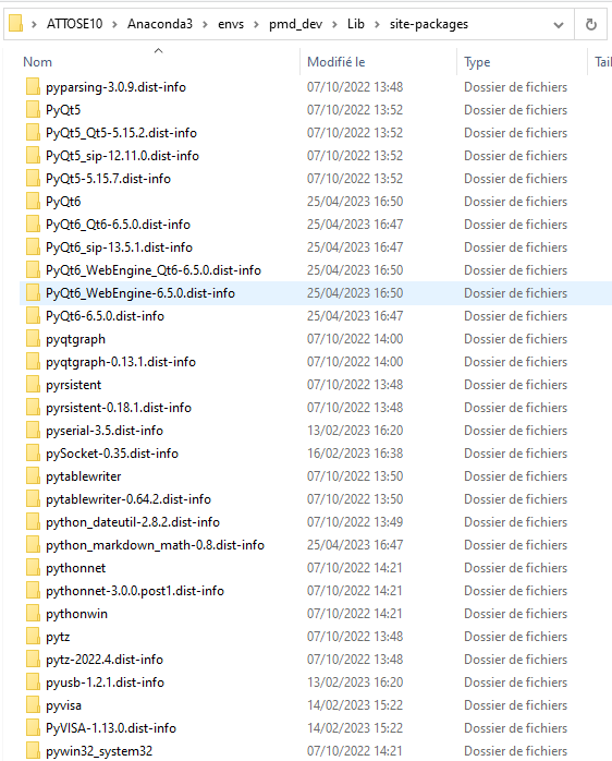
Fig. 5.44 Content of the site-packages folder of our pmd_dev environment.

The subfolders that you find inside correspond to the Python packages that are installed within this environment. A general rule is that you should never modify manually anything in this folder. Those folders contain the exact versions of each package that is installed in our environment. If we modify them in a dirty way (not versioned), we will very fast loose the control about our modifications. The edition option “-e” of pip is the solution to work in a clean way, it allows to simulate that our package is installed in the environment. This way, during the development period of our plugin, we can safely do any modification in our folder C:\Users\<OS username>\local_repository\pymodaq_plugins_physik_instrumente (refered to by the “.” in the command) and it will behave as if it was in the site-packages. To check that this last command executed properly, you can check that you have a file called pymodaq_plugins_physik_instrumente.egg-link that has been created in the site-packages folder. Note that pip knows with which Python environment to deal with because we have activated pmd_dev.

5.4.6.5. Open the package with an adapted IDE

In this section we will work not only with a simple script, but within a Python project that contains multiple files and that is much more complex than a simple script. For that Spyder is not so well adapted. In this section we will present PyCharm because it is free and very powerful, but you can probably found an equivalent one.

Once it is opened, go to File > New project. Select the repository folder and the Python interpreter.

Fig. 5.45 Start a project with PyCharm. You have to select the main folder that you will work with, and the Python interpreter corresponding to your environment.

You can for example configure the interface so that it looks like the following figure.

Fig. 5.46 PyCharm interface. Left panel: tree structure of the folders that are included in the PyCharm project. Center: edition of the file. Right panel: structure of the file. Here you found the different methods and argument of the Python class that are defined in the file. Bottom: different functionalities that are extremely usefull: a Python console, a terminal, a debugger, integration of Git…

In the left panel, you will find the folder corresponding to our repository, so that you can easily open the files you are interested in. We will also add in the project the PyMoDAQ core folder, so that we can easily call some entry points of PyMoDAQ. To do so, go to File > Open and select the PyMoDAQ folder. Be careful to not get lost in the tree structure, you have to go select the select the folder that is in the good environment. In this case C:\Users\<OS username>\Anaconda3\envs\pmd_dev\Lib\site-packages\pymodaq (in particular, do not mistake with the site-packages of the base Anaconda environment that is located at C:\Users\<OS username>\Anaconda3\Lib\site-packages), click OK and then Attach.

The pymodaq folder should now appear in the left panel, navigate within it, open and Run (see figure) the file pymodaq > daq_move > daq_move_main.py. This is equivalent to execute the daq_move command in a terminal. Thus you should now see the GUI of the DAQ_Move.

5.4.6.6. Debug of the original plugin

As we have noticed before, a lot of things where already working in the original plugin. It is now time to analyse what is happening. For that, we will use the debbuger of our IDE, which is an indispensable to debug PyMoDAQ. You will save a lot of time by mastering this tool! And it is very easy to use.

Let us now open the daq_move_PI.py file. This file defines a class corresponding to the original PI plugin, and you can have a quick look at the methods inside using the Structure panel of PyCharm. Basically, most of the methods of the class are triggered by a button from the user interface, as is illustrated in the following figure.

Fig. 5.47 Each action of the user on the UI triggers a method of the instrument class.

During our first test of the plugin, earlier in this tutorial, we noticed that things went wrong at the moment we click the Initialize button, which correspond to the ini_stage method of the DAQ_Move_PI class. We will place inside this method some breakpoints to analyse what is going on. To do so, you just have to click within the breakpoints column at the lign you are interested in. A red disk will appear, as illustrated by the next capture.

Fig. 5.48 See the breakpoints inside your PyCharm project.

When you run a file in DEBUG mode (bug button instead of play button), it means that PyCharm will execute the file until it finds an activated breakpoint. It will then stop the execution and wait for orders: you can then resume the program up to the next breakpoint, or execute lign by lign, rerun the program from the begining…

When you run the DEBUG mode, notice that a new Debug panel appears at the bottom of the interface. The View breakpoints button will popup a window so that you see where are the breakpoints within all your PyCharm project, that is to say within all the folders that you attached to your project, and that are present in the tree structure of the Project panel. You can also deactivate a breakpoint, in that case it will be notified with a red circle.

Fig. 5.49 Execute PyMoDAQ in DEBUG mode.

Let us now run in DEBUG mode the daq_move_main.py file. We select the PI plugin (not the PI E870), the good controller, and initialize. PyCharm stops the execution at the first breakpoint and highlight the corresponding lign in the file. This way we progress step by step up to “sandwitching” the lign that triggers the error with breakpoints. Looking at the value of the corresponding variable, we found again the Unknown command (2) error message that we already had in the PyMoDAQ log file.

Fig. 5.50 Find the buggy line. The breakpoint lign 163 is never reached. The value of the self.controller.gcscommands.axes variable is Unknown command (2).

Let’s go there to see what happens. We can attach the pipython package to our PyCharm project and look at this axes attribute. In this method we notice the call to the qSAI method, which is NOT supported by our controller! We now have a precise diagnosis of our bug :)

Fig. 5.51 The axes attribute calls the SAI? GCS command that is not supported by the E870 controller.

5.4.6.7. Write the class for our new instrument

Coding a PyMoDAQ plugin actually consists in writting a Python class with specific conventions such that the PyMoDAQ core knows where to find the installed plugins and where to call the correct methods.

The PyMoDAQ plugins template repository is here to help you follow those conventions and such that you have to do the minimum amount of work. Let see what it looks like!

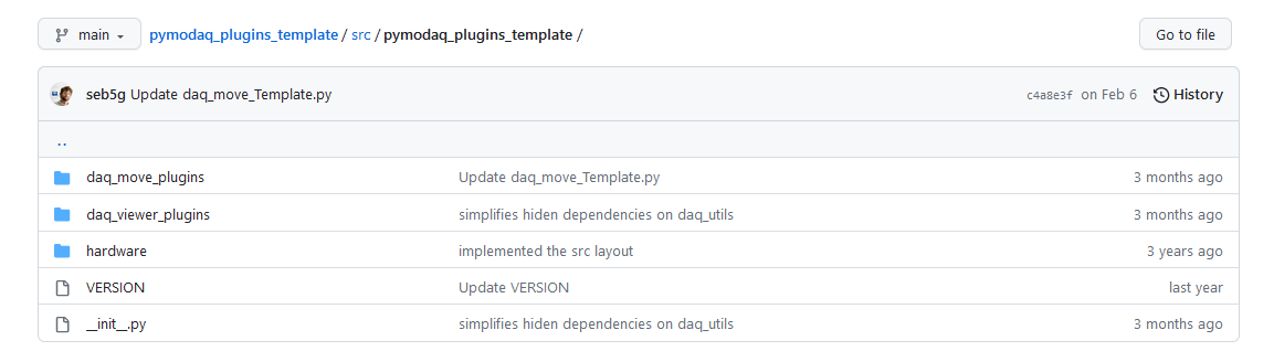
Fig. 5.52 Tree structure of the plugin template repository.

The src directory of the repository is subdivided into three subfolders

• daq_move_plugins which stores all the instruments corresponding to actuators.

• daq_viewer_plugins, which stores all the instruments corresponding to detectors. It is itself divided into subfolders corresponding to the dimensionality of the detector.

• hardware, within which you will find Python wrappers (optional).

Within each of the first two subfolders, you will find a Python file defining a class. In our context we are interested in the one that is defined in the first subfolder.

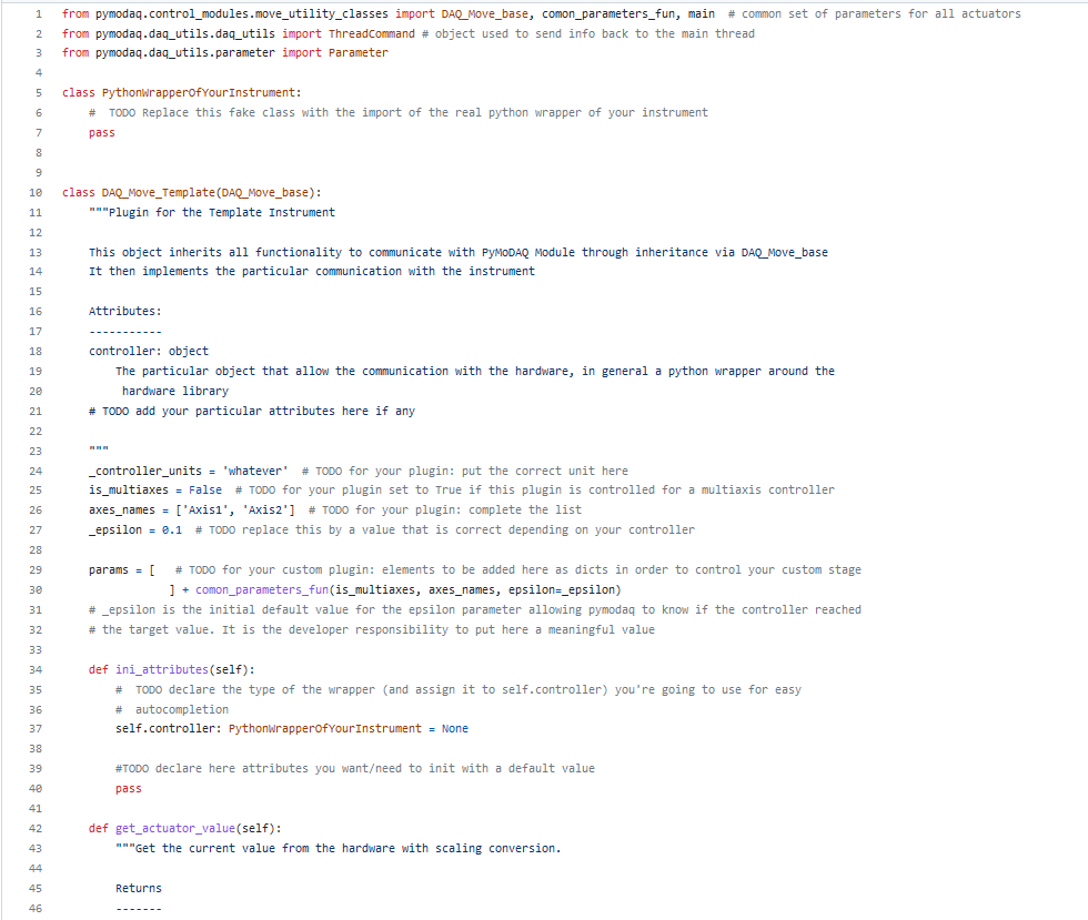
Fig. 5.53 Definition of the DAQ_Move_Template class.

As you can see the structure of the instrument class is already coded. What we have to do is to follow the comments associated to each line, and insert the scripts we have developped in a previous section (see gold route) in the right method.

There are naming conventions that should be followed:

• We already mentioned that the name of the package should be pymodaq-plugins-<company name>. Do not forget the “s” at “plugins” ;)

• The name of the file should be daq_move_xxx.py and replace xxx by whatever you like (something that makes sense is recommended ;) )

• The name of the class here should be DAQ_Move_xxx.

• The name of the methods that are already present in the template should be kept as it is.

Note

Be careful that in the package names, the separator is “-”, whereas in file names, the separator is “_”.

The name of the methods is quite explicit. Moreover, the docstrings are here to help you understand what is expected in each method.

Note

In Python, a method’s name should be lowercase.

Go to the daq_move_plugins folder, you should find some files like daq_move_PI.py, which correspond to the other plugins that are already present in this package.

With a right click, we will create a new file in this folder that we will call daq_move_PI_E870.py. Copy the content of the daq_move_Template.py file and paste it in the newly created file.

Change the name of the class to DAQ_Move_PI_E870.

Run again the daq_move_main.py file.

You should now notice that our new instrument is already available in the list! This is thanks to the naming conventions. However, the initialization will obviously fail, because for now we did not input any logic in our class.

Before we go further, let us configure a bit more PyCharm. We will first fix the maximum number of characters per lign. Each Python project fixes its own convention, so that the code is easier to read. For PyMoDAQ, the convention is 120 characters. Go to File > Settings > Editor > Code Style and configure Hard wrap to 120 characters.

Introduction of the class

We call the introduction of the class the code that is sandwitched between the class keyword and the first method definition. This code will be executed after the user selected the instrument he wants to use through the DAQ_Move UI.

This part of the code from the original plugin was working, so let’s just copy-paste it, and adapt a bit to our case.

Fig. 5.54 Introduction of the class of our PI E870 instrument.

First, it is important that we comment the context of this file, this can be done in the docstring attach to the class, PyMoDAQ follows the Numpy style for its documentation

Notice that the import of the wrapper is very similar to what we have done in the gold route. However, we do not call anymore the InterfaceSetupDlg() method that was poping up a window. We rather use the EnumerateUSB() method to get the list of the addresses of the plugged controllers, which will then be sent in the parameter panel (in the item named Devices) of the DAQ_Move UI. We now understand precisely the sequence of events that makes the list of controller addresses available just after we have selected our instrument.

Notice that in the class declaration not all the parameters are visible. Most of them are declared in the comon_parameters_fun that declares all the parameters that are common to every plugin. But if at some point you need to add some specific parameter for your instrument, you just have to add an element in this params list, and it will directly be displayed and controllable through the DAQ_Move UI! You should fill in a title, a name, a type of data, a value … You will find this kind of tree everywhere in the PyMoDAQ code. Copy-paste the first lign for exemple and see what happens when you execute the code ;)

To modify the value of such a parameter, you will use something like

self.settings.child('multiaxes', 'axis').setValue(2)

Here we say “in the parameter tree, choose the axis parameter, in the multiaxes group, and attribute him the value 2 “

Note

self.settings is a Parameter object of the pyqtgraph library.

Get the value of this parameter will be done with

self.settings['multiaxes', 'axis']

ini_stage method

As mentioned before, the ini_stage method is triggered when the user click the Initialization button. It is here that the communication with the controller is established. If everything works fine, the LED will turn green.

Fig. 5.55 ini_stage method of our PI E870 instrument class.

Compared to the initial plugin, we simplified this method by removing the functions that were intended for close-loop operation. Plus we only consider the USB connexion. The result is that our controller initializes correctly now: the LED is green!

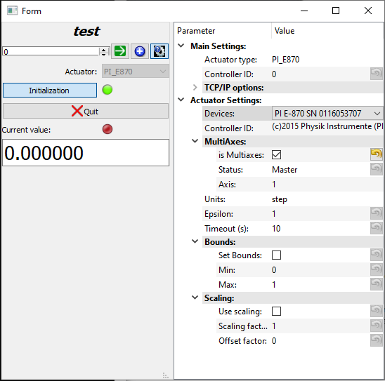
Fig. 5.56 Now our controller initializes correctly.

commit_settings method

Another important method is commit_settings. This one contains the logic that will be triggered when the user modifies some value in the parameter tree. Here will be implemented the change of axis of the controller, by changing the configuration of the demultiplexer with the MOD GCS command (see the gold route).

Fig. 5.57 commit_settings method of our PI E870 instrument class. Implementation of a change of axis.

move_rel method

Finally, the move_rel method, that implements a relative move of the actuator is quite simple, we just use the OSM command that we found when we studied the DLL with a simple script.

Fig. 5.58 move_rel method of our PI E870 instrument class. Implementation of a relative move.

We can now test the Rel + / Rel - buttons, a change of axis… it works!

There is still minor methods to implement, but now you master the basics of the instrument plugin development ;)

5.4.6.8. Commit our changes with Git

Now that we have tested our changes, we can be happy with this version of our code. We will now stamp this exact content of the files, so that in the future, we can at any time fall back to this working version. You should see Git as your guarantee that you will never lost anything of your work.

At the location of our local repository, we will now use this Git command

C:\Users\<OS username>\local_repository\pymodaq_plugins_physik_instrumente>git diff

you should get something that looks like this

Fig. 5.59 Answer to the git diff command in a terminal. Here are the modifications of the daq_move_PI_E870.py file. In red are the lines that have been deleted, in green the lines that have been added.

This Git command allows us to check precisely the modifications we have done, which is called a diff.

In the language of Git, we stamp a precise state of the repository by doing a commit

C:\Users\<OS username>\local_repository\pymodaq_plugins_physik_instrumente>git commit -am "First working version of the E870 controller plugin."

Within the brackets, we leave a comment to describe the changes we have made.

Then, with the git log command, you can see the history of the evolution of the repository

C:\Users\<OS username>\local_repository\pymodaq_plugins_physik_instrumente>git log

Fig. 5.60 Answer to the git log command in a terminal.

5.4.6.9. Push our changes to our remote repository

We have now something that is working locally. That is great, but what if at some point, the computer of my experiment suddenly crashes? What if I want to share my solution to a collegue that have the same equipment?

Would not it be nice if I could command my controller on any machine in the world with a few command lines? :O

It is for those kind of reasons that it is so efficient to work with a remote server. It is now time to benefit from our careful preparation! Sending the modifications on our remote repository is done with a simple command

C:\Users\<OS username>\local_repository\pymodaq_plugins_physik_instrumente>git push

In the Git vocabulary, pushing means that you send your work to your remote repository. If we go on our remote server on GitHub, we can notice that our repository has actually been updated!

Fig. 5.61 The git push command updated our remote repository.

From now on, anyone who has an internet connexion have access to this precise version of our code.

Note

You may wonder how Git knows where to push? This has been configured when we cloned our remote repository. You can ask what is the current address configured of your remote repository (named origin) with the git remote -v command.

5.4.6.10. Pull request to the upstream repository

But this is not the end! Since we are very proud of our new plugin, why not make all the users of PyMoDAQ benefit from it? Why not propose our modification to the official pymodaq_plugin_physik_instrumente repository?

Again, since we prepared properly, it is now a child play to do that. In the Git vocabulary, we say that we will do a pull request, often abreviated as PR. This can be done through the interface of GitHub. Log in to your account, go to the repository page and click, in the Pull request tab, the Create pull request button.

You have to be careful to select properly the good repositories and the good branches. Remember that in our case we created a E-870 branch.

Fig. 5.62 The GitHub interface to create a PR.

Leave a message to describe your changes and submit. Our pull request is now visible on the upstream repository.

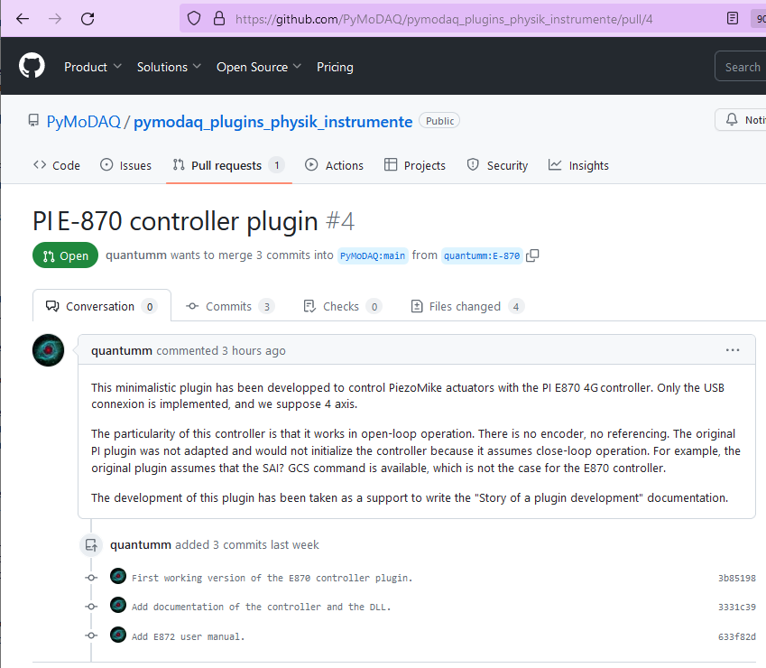
Fig. 5.63 Our pull request in the upstream repository.

This opens a space where you can discuss your changes with the owner of the repository. It will be his decision to accept or not the changes that we propose. Let us hope that we will convince him! :) Often these discussions will lead to a significant improvement of the code.

5.4.7. Conclusion

That’s it!

We have tried, with this concrete example, to present the global workflow of an instrument plugin development, and the most common problems you will face. Do not forget that you are not alone: ask for help, it is an other way to meet your collegues!

We have also introduce a software toolbox for Python development in general, that we sum up in the following table. They are all free of charge. Of course this is just a suggestion, you may prefer different solutions. We wanted to present here the main types of software you need to develop efficiently.

Software function	Solution presented
Python environment manager	Anaconda
Python package manager	pip
Python IDE	Spyder / PyCharm
Version control software	Git
Repository host	GitHub

Finally, remember that while purchasing an instrument, it is important to check what your supplier provides as a software solution (Python wrapper, Linux drivers…). This can save you a lot of time!