3.6.1. What is PyMoDAQ’s Data?
Data in PyMoDAQ are objects with many characteristics:
a type: float, int, …
a dimensionality: Data0D, Data1D, Data2D and we will discuss about DataND
units
axes
actual data as numpy arrays
uncertainty/error bars
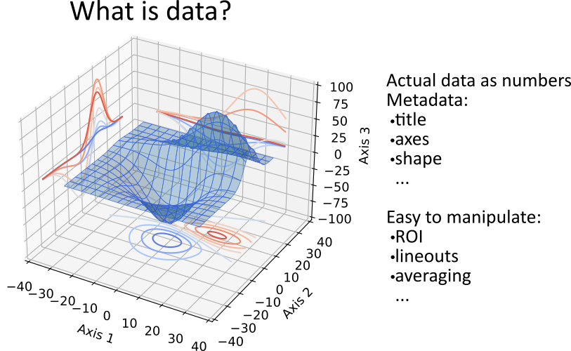
Fig. 3.52 What is PyMoDAQ’s data?.
Because of this variety, PyMoDAQ introduce a set of objects including metadata (for instance the time of acquisition)
and various methods and properties to manipulate those (getting name, slicing, concatenating…). The most basic object
is DataLowLevel whose all data objects will inherit. It is very basic and will only store a name as a string and a
timestamp from its time of creation.
Then one have DataBase objects that stores homogeneous data (data of same type) having the same shape as a list of numpy arrays.
Numpy is fundamental in python and it was obvious to choose that. However, instruments can acquire data having the same type and shape but from different channels. It then makes sense to have a list of numpy arrays.
Figure Fig. 3.53 presents the different types of data objects introduced by PyMoDAQ, which are also described below with examples on how to use them.
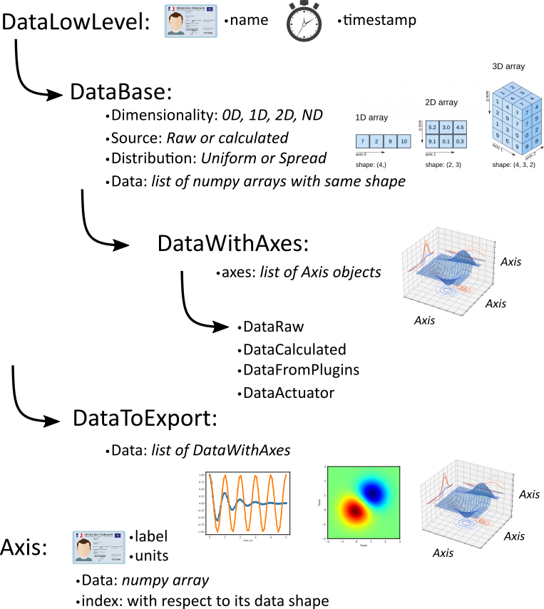
Fig. 3.53 Zoology of PyMoDAQ’s data objects.
3.6.1.1. DataBase
DataBase, see Data Management, is the most basic object to store data (it should in fact not be used for real cases, please use DataWithAxes). It takes as argument a name, a DataSource, a DataDim, a DataDistribution, the actual data as a list of numpy arrays (even for scalars), labels (a name for each element in the list), eventually an origin (a string from which module it originates) and optional named arguments.
>>> import numpy as np
>>> from pymodaq.utils.data import DataBase, DataSource, DataDim, DataDistribution
>>> data = DataBase('mydata', source=DataSource['raw'],\
distribution=DataDistribution['uniform'], data=[np.array([1,2,3]), np.array([4,5,6])],\
labels=['channel1', 'channel2'], origin="documentation's code")
When instantiated, some checks are performed:
checking the homogeneity of the data
the consistency of the dimensionality and the shape of the numpy arrays
if no dimensionality is given, it is inferred from the data’s shape
Useful properties can then be used to check and manipulate the data. For instance one can check the length of the object (number of numpy arrays in the list), the size (number of elements in the numpy arrays), the shape (shape of the numpy arrays).
>>> data.dim
<DataDim.Data1D: 1>
>>> data.source
<DataSource.raw: 0>
>>> data.shape
(3,)
>>> data.length
2
>>> data.size
3
One can also make mathematical operations between data objects (sum, substraction, averaging) or appending numpy arrays (of same type and shape) to the data object and iterating over the numpy arrays with the standard for loop.
>>> for subdata in data:
      print(subdata)
      print(subdata.shape)
[1 2 3]
(3,)
[4 5 6]
(3,)
For a full description see What is PyMoDAQ’s Data?.
Of course for data that are not scalar, a very important information is the axis associated with the data (one axis for waveforms, two for 2D data or more for hyperspectral data). PyMoDAQ therefore introduces Axis and DataWithAxes objects.
3.6.1.2. Axis
The Axis object stores the information about the data’s axis
>>> from pymodaq.utils.data import Axis
>>> axis = Axis('myaxis', units='seconds', data=np.array([3,7,11,15]), index=0)
>>> axis
Axis: <label: myaxis> - <units: seconds> - <index: 0>
It has a name, units, actual data as a numpy array and an index referring to which dimension of Data
the axis is referring to. For example, index=0 for the vertical axis of 2D data and index=1 for the
horizontal (or inversely, it’s up to you…).
Because there is no need to store a linearly spaced array, when instantiated, the Axis object will, for linear
axis’s data replace it by None but compute an offset and a scaling factor
>>> axis.data
None
>>> axis.offset
3
>>> axis.scaling
4.0
>>> axis.size
4
Axis object has also properties and methods to manipulate the object, for instance to retrieve the associated numpy array:
>>> axis.get_data()
array([ 3.,  7., 11., 15.])
and mathematical methods:
>>> axis.mean()
11.0
>>> axis.find_index(11.0)
2
and a special slicer property to get subparts of the axis’s data (but as a new Axis object):
>>> axis.iaxis[2:].get_data()
array([11., 15.])
3.6.1.3. DataWithAxes
When dealing with data having axes (even 0D data can be defined as DataWithAxes),
the DataBase object is no more enough to describe the data.
PyMoDAQ therefore introduces DataWithAxes which inherits from DataBase and introduces more
metadata and functionalities.
>>> from pymodaq.utils.data import DataWithAxes
>>> data = DataWithAxes('mydata', source=DataSource['raw'], dim=DataDim['Data2D'], \
distribution=DataDistribution['uniform'], data=[np.array([[1,2,3], [4,5,6]])],\
axes=[Axis('vaxis', index=0, data=np.array([-1, 1])),
Axis('haxis', index=1, data=np.array([10, 11, 12]))])
>>> data
<DataWithAxes, mydata, (|2, 3)>
>>> data.axes
[Axis: <label: vaxis> - <units: > - <index: 0>,
 Axis: <label: haxis> - <units: > - <index: 1>]
This object has a few more methods and properties related to the presence of axes. It has in particular an
AxesManager attribute that deals with the Axis objects and the Data’s representation (|2, 3)
Here meaning the data has a signal shape of (2, 3). The notion of signal will be highlighted in the next
paragraph.
It also has a slicer property to get subdata:
>>> sub_data = data.isig[1:, 1:]
>>> sub_data.data[0]
array([5, 6])
>>> sub_data = data.isig[:, 1:]
>>> sub_data.data[0]
array([[2, 3],
       [5, 6]])
3.6.1.4. Uncertainty/error bars
The result of a measurement can be captured through averaging of several identical data. This batch of data can be saved as a higher dimensionality data (see DAQ Scan averaging). However the data could also be represented by the mean of this average and the standard deviation from the mean. DataWithAxes introduces therefore this concept as another object attribute: errors.
data = DataWithAxes('mydata', source=DataSource['raw'], dim=DataDim['Data1D'],
                    data=[np.array([1,2,3])],
                    axes=[Axis('axis', index=0, data=np.array([-1, 0, 1])),
                    errors=[np.array([0.01, 0.03, 0,1])])
The errors parameter should be either None (default) or a list of numpy arrays (list as long as there are data numpy arrays) having the same shape as the actual data.
3.6.1.6. Uniform and Spread Data
So far, everything we’ve said can be well understood for data taken on a uniform grid (1D, 2D or more). But
some scanning possibilities of the DAQ_Scan (Tabular) allows to scan on specifics (and possibly random) values
of the actuators. In that case the distribution is DataDistribution['spread']. Such distribution will be
differently plotted and differently saved in a h5file. It’s dimensionality will be DataND and a specific AxesManager
will be used. Let’s consider an example:
One can take images data (20x30 pixels) as a function of 2 parameters, say xaxis and yaxis non-uniformly spaced
>>> data.shape = (150, 20, 30)
>>> data.nav_indexes = (0,)
The first dimension (150) corresponds to the navigation (there are 150 non uniform data points taken) The second and third correspond to signal data, here an image of size (20x30 pixels) so:
nav_indexesis (0, )sig_indexesis (1, 2)
>>> xaxis = Axis(name=xaxis, index=0, data=...)
>>> yaxis = Axis(name=yaxis, index=0, data=...)
both of length 150 and both referring to the first index (0) of the shape
In fact from such a data shape the number of navigation axes is unknown . In our example, they are 2. To somehow
keep track of some ordering in these navigation axes, one adds an attribute to the Axis object: the spread_order
>>> xaxis = Axis(name=xaxis, index=0, spread_order=0, data=...)
>>> yaxis = Axis(name=yaxis, index=0, spread_order=1, data=...)
This ordering will be very important for plotting of the data, see for instance below for an adaptive scan:
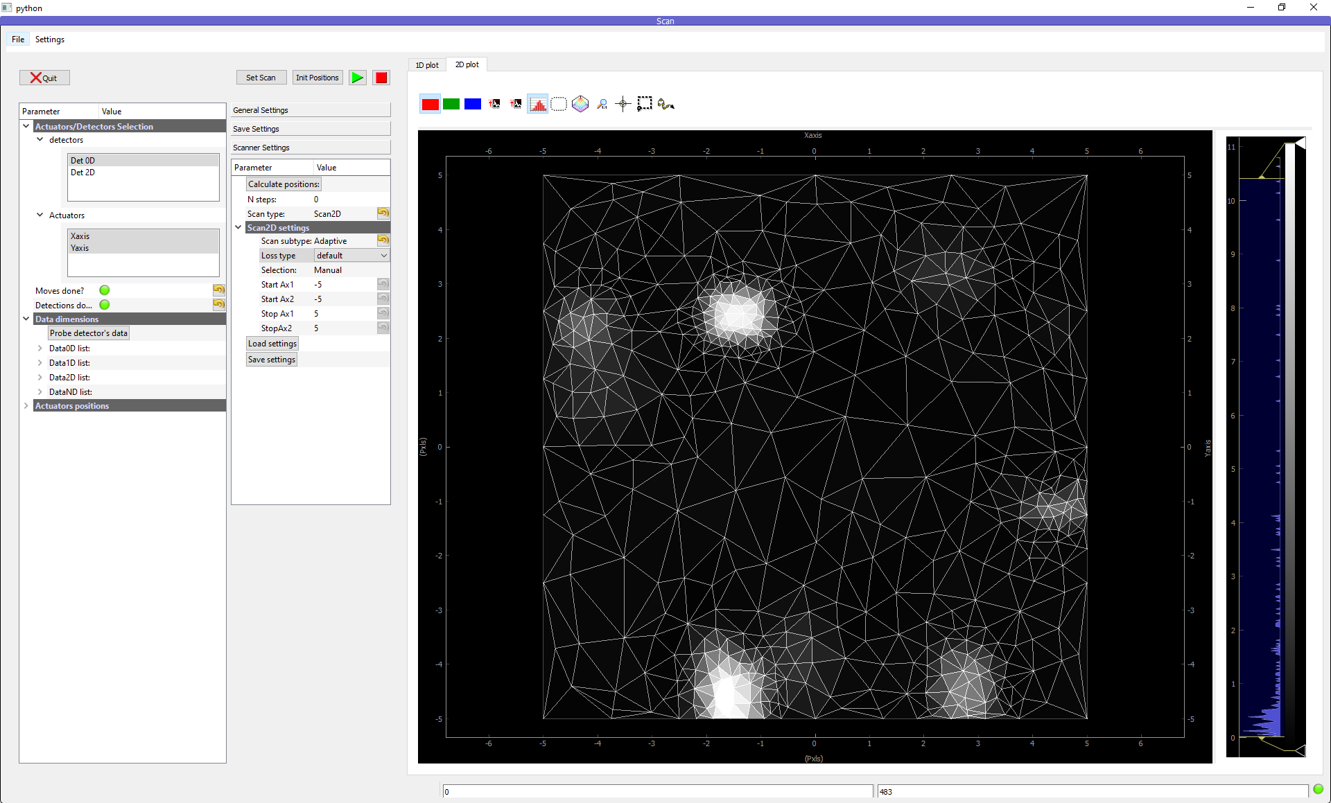
Fig. 3.54 Non uniform 2D plotting of Spread DataWithAxes.
3.6.1.7. Special DataWithAxes
For explicit meaning, several classes are inheriting DataWithAxes with adhoc attributes such as:
DataRaw:DataWithAxeswith its source set toDataSource['raw']DataFromPlugins: explicitDataRawto be used within Instrument pluginsDataCalculated:DataWithAxeswith its source set toDataSource['calculated']DataFromRoi: explicitDataCalculatedto be used when processing data using ROI.
3.6.2. DataToExport
In general a given instrument (hence its PyMoDAQ’s Instrument plugin) will generate similar data (for instance several
Data1D waveforms for each channel of an oscilloscope). Such data can be completely defined using DataWithAxes as we
saw above.
However, when then plotting such data, the user can decide to use ROI to extract some meaningfull information to be
displayed in a live DAQ_Scan plot. This means that the corresponding DAQ_Viewer will produce both Data1D’s data but also
several Data0D’s ones depending on the number of used ROIs. To export (emit signals) or save (to h5), it would be much
better to have a specialized object to deal with these non-similar data. This is the role of the DataToExport
object.
DataToExport is a DataLowLevel object with an extra attribute data, that is actually a list of DataWithAxes
objects:
>>> from pymodaq.utils.data import DataToExport, DataRaw
>>> dwa0D = DataRaw('dwa0D', data=[np.array([1]), np.array([2]) , np.array([3])])
>>> dwa1D = DataRaw('dwa1D', data=[np.array([1, 2 , 3])])
>>> dte = DataToExport(name='a_lot_of_different_data', data=[dwa0D, dwa1D])
>>> dte
DataToExport: a_lot_of_different_data <len:2>
It has a length of 2 because contains 2 DataWithAxes objects (dwa). One can then easily get the data from it :
>>> dte[0]
<DataRaw, dwa0D, (|1)>
or get dwa from their dimensionality, their name, the number of axes they have …
>>> dte.get_data_from_dim('Data1D').data[0]
<DataRaw, dwa1D, (|3)>
>>> dte.get_names()
['dwa0D', 'dwa1D']
>>> dte.get_data_from_name('dwa0D')
<DataRaw, dwa0D, (|1)>
Dwa can also be appended or removed to/from a DataToExport.
For more details see Union of Data