3.5.1.5. Scanner
The Scanner module is an object dealing with configuration of scan modes and is mainly used by the DAQ_Scan extension. It features a graphical interface, see Fig. 3.30, allowing the configuration of the scan type and all its particular settings. The Scan type sets the type of scan, Scan1D for a scan as a function of only one actuator, Scan2D for a scan as a function of two actuators, Sequential for scans as a function of 1, 2…N actuators and Tabular for a list of points coordinates in any number of actuator phase space. All specific features of these scan types are described below:
3.5.1.5.1. Scan1D
The possible settings are visible on Fig. 3.29 and described below:
scan subtype: either Linear (usual uniform 1D scan), Back to start (the actuator comes back to the initial position after each linear step, for a referenced measurement for instance), Random same as Linear except the predetermined positions are sampled randomly and from version 2.0.1 Adaptive that features no predetermined positions. These will be determined by an algorithm influenced by the signal returned from a detector on the previously sampled positions (see Adaptive)
Start: Initial position of the selected actuator (in selected actuator controller unit)
Stop: Last position of the scan (in selected actuator controller unit)
Step: Step size of the step (in selected actuator controller unit)
For the special case of the Adaptive mode, one more feature is available: the Loss type*. It modifies the algorithm behaviour (see Adaptive)
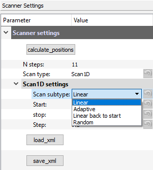
Fig. 3.29 The Scanner user interface set on a Scan1D scan type and the visible list of scan subtype.
3.5.1.5.2. Scan2D
The possible settings are visible on Fig. 3.30 and described below:
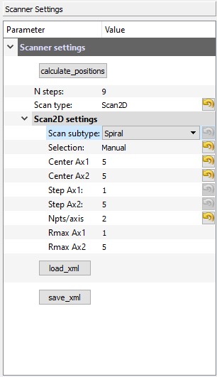
Fig. 3.30 The Scanner user interface set on a Scan2D scan type and a Spiral scan subtype and its particular settings.
Scan subtype: See Fig. 3.31 either linear (scan line by line), linear back and forth (scan line by line but in reverse direction each 2 lines), spiral (start from the center and scan as a spiral), Random (random sampling of the linear case) and Adaptive (see Adaptive)
Start, Stop, Step: for each axes (each actuators)
Rmax, Rstep, Npts/axis: in case of spiral scan only. Rmax is the maximum radius of the spiral (calculated), and Npts/axis is the number of points for both axis (total number of points is therefore Npts/axis²).
Selection: see Scan Selector
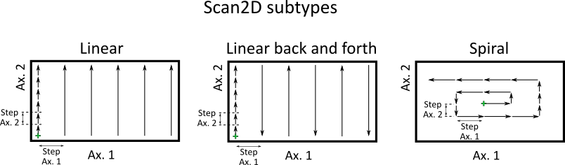
Fig. 3.31 The main Scan2D subtypes: Linear, Back and Forth and Spiral.
3.5.1.5.3. Sequential
The possible settings are visible on Fig. 3.32 and described below:
Scan subtype: only linear this means the scan have a sequence of Scan1D of the last specified actuator (on Fig. 3.32, it is Xaxis) for all positions of the last but end actuator (here Yaxis) and so on. So on Fig. 3.32 there will be 11 steps for Xaxis times 11 steps for Yaxis times 10 steps for Theta axis so in total 11x11x10=1210 total steps for this 3 dimensions scan.
Note
If only 1 actuator is selected, then the Sequential scan is identical to the Scan1D scan but where only the linear subtype is available. If 2 actuators are selected, then the Sequential scan is identical to the Scan2D scan but where only the linear subtype is available.
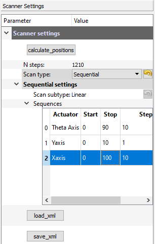
Fig. 3.32 The Scanner user interface set on a Sequential scan type with a sequence of three actuators
3.5.1.5.4. Tabular
The tabular scan type consists of a list of positions (for each selected actuators).
3.5.1.5.4.1. Tabular Linear/Manual case
In the Linear/Manual case, the module will move actuators on each positions and grab datas. On Fig. 3.33, a list of 79 positions has been set. By right clicking on the table, a context manager pops up and gives the possibility to:
add one more position in the list
remove the selected position
clear all the positions
load positions from a text file (as many columns as selected actuators with their positions separated by a tab)
save the current list of positions in a text file (for later quick loading of positions)
One can also drag and drop elements of the list at a different index in the list.
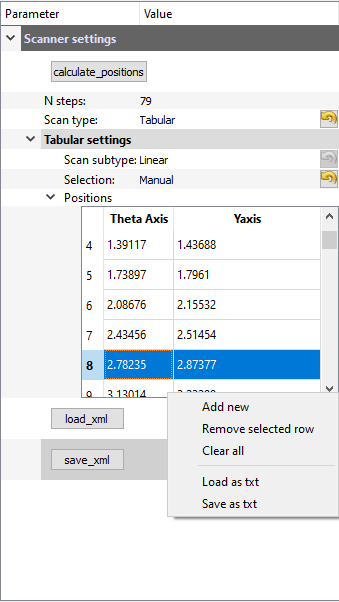
Fig. 3.33 The Scanner user interface set on a Tabular scan type with a list of points for 2 actuators. A context menu with other options is also visible (right click on the table to show it)
3.5.1.5.4.2. Tabular Linear/Polylines case
In the particular case of 2 selected actuators, it could be more interesting to draw the positions for the tabular scan. One possibility is to draw segments on a 2D viewer (see Fig. 3.34) and positions will be points along these segments (it will be a kind of 1D cuts within a 2D phase space). A new setting, Curvilinear step appears. The positions will be points starting from the start of the first segment and then step along them by the value of this setting. That gives, for Fig. 3.34, 40 points defined along the segments.
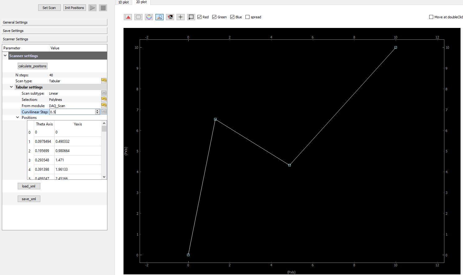
Fig. 3.34 An example of 1D complex sections selected within a 2D area
3.5.1.5.4.3. Tabular Adaptive case
Valid for 1 or 2 selected actuators. The tabular adaptive case will be similar to scan1D adaptive mode, except that one adaptive Scan1D will be done for each segments defined by the list of positions in the table. For instance, Fig. 3.35 shows a list of 4 positions defining 4 segments in a 2D space. The adaptive scan will be done on/along these 4 segments. Positions can be set manually or from a Polylines selection as seen on Fig. 3.34.
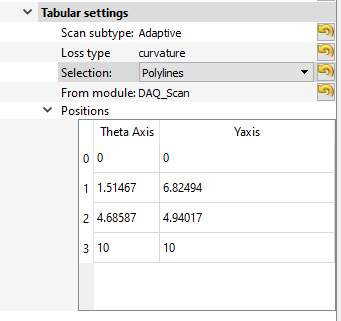
Fig. 3.35 The Scanner user interface set on a Tabular scan type with a list of points for 2 actuators. A context menu with other options is also visible (right click on the table to show it)
3.5.1.5.5. Adaptive
All the adaptive features are using the python-adaptive package (Parallel active learning of mathematical functions, 10.5281/zenodo.1182437). And the reader is invited to explore their tutorials to discover how these algorithms work. In PyMoDAQ the learner1D algorithm is used for the Scan1D and Tabular scan types while the learner2D one is used for Scan2D scan type.
3.5.1.5.5.1. Bounds
As a general rule, the adaptive algorithm will need bounds to work with. For Scan1D scan type, these will be defined from the start and stop settings. For Tabular, it is the start and ends of the segments. Finally for Scan2D, it is the: Start Ax 1, Stop Ax 1 and Start Ax 2, Stop Ax 2 that are defining scan bounds.
3.5.1.5.5.2. Feedback
The adaptive algorithm will need for each probed positions a feedback value telling it the fitness of the probed points. From these on all previous points, it will determine the best next points to probe. In order to provide such a feedback, on has to choose a signal among all available from the DashBoard detectors. It has to be a Scalar so originate from a 0D detector or integrated ROI from 1D or 2D detectors. The module manager user interface (right most setting tree in the DAQ_Scan module ,see Fig. 3.84) will let you probe available datas exported from currently selected detectors. You can then pick the Data0D one you want to use as the Adaptive feedback. For instance, on Fig. 3.84, three Data0D are available, one from a 0D detector (CH000) and 2 from the Measurements ROIs of a 1D detector. In that case the CH000 data has been selected and will therefore be use as feedback for the Adaptive algorithm.
3.5.1.5.5.3. Loss
All the Adaptive options are called Loss on the Scanner UI. These influence the adaptive algorithm, using previously probed positions and their feedback to guess the next point to probe. See the Adaptive documentation on loss to understand all the possibilities.