3.5.1.1. Introduction
The dashboard gives you full control for manual adjustments (using the UI)
of each actuator, checking their impact on live data from the detectors. Once all is set, one can move to
an automated scan using the main control window of the DAQ_Scan, see Fig. 3.20.
3.5.1.2. Main Control Window
The main control window is comprised of various panels to set all parameters and display live data taken during a scan.

Fig. 3.20 Main DAQ_Scan user interface.
The instrument selection panel allows to quickly select the detectors and the actuators to use for the next scan
The settings panel is divided in three sections (see Settings for more details):
Scanner settings: select and set the next scan type and values.
General settings: options on timing, scan averaging and plotting.
Save settings: everything about what should be saved, how and where.
The Live plots selection panel allows to select which data produced from selected detectors should be rendered live
The Live Plots panels renders the data as a function of varying parameters as selected in the Live plots selection panel
3.5.1.3. Scan Flow
Performing a scan is typically done by:
Selecting which detectors to save data from
Selecting which actuators will be the scan varying parameters
Selecting the type of scan (see Selecting the type of scan): 1D, 2D, … and subtypes
For a given type and subtype, settings the start, stop, … of the selected actuators
Selecting data to be rendered live (none by default)
Starting the scan
3.5.1.3.1. Selecting detectors and actuators
The Instrument selection panel is the user interface of the module manager (see Module Manager for details).
It allows the user to select the actuators and detectors for the next scan (see Fig. 3.21). This interface
is also used for the DAQ_Logger extension.
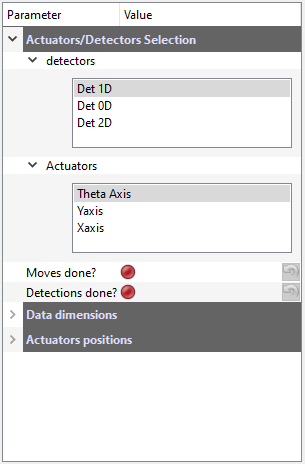
Fig. 3.21 List of declared modules from a preset
3.5.1.3.2. Selecting the type of scan
All specifics of the upcoming scan are configured using the scanner_paragrah module interface as seen on Fig. 3.22 in the case of a spiral Scan2D scan configuration.
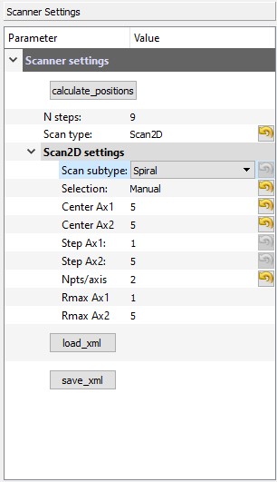
Fig. 3.22 The Scanner user interface set on a Scan2D scan type and an adaptive scan subtype and its particular settings.
3.5.1.3.3. Selecting the data to render live
For a data acquisition system to be efficient, live data must be plotted in order to follow the experiment behaviour and check if something is going wrong or successfully without the need to perform a full data analysis. For this PyMoDAQ live data display will allows the user to select data to be plotted from the selected detectors.
The list of all possible data to be plotted can be obtained by clicking on the  button. All data will
be classified by dimensionality (0D, 1D). The total dimensionality of the data + the scan dimensions
(1 for scan1D and 2 for Scan2D…) should not exceed 2 (this means one cannot plot more complex plots than 2D intensity
plots). It also means that you should use ROI to generate lower dimensionality data from your raw data for a proper
live plot.
button. All data will
be classified by dimensionality (0D, 1D). The total dimensionality of the data + the scan dimensions
(1 for scan1D and 2 for Scan2D…) should not exceed 2 (this means one cannot plot more complex plots than 2D intensity
plots). It also means that you should use ROI to generate lower dimensionality data from your raw data for a proper
live plot.
For instance, if the chosen detector is a 1D one, see Fig. 3.23. Such a detector can generate various type of live data.

Fig. 3.23 An example of a 1D detector having 2 channels. 0D data are generated as well from the integration of channel CH0 within the regions of interest (ROI_00 and ROI_01).
It will export the raw 1D data and the 1D lineouts and integrated 0D data from the declared ROI as shown on Fig. 3.24

Fig. 3.24 An example of all data generated from a 1D detector having 2 channels. 0D data and 1D data are generated as well from the integration of channel CH0 within the regions of interest (ROI_00 and ROI_01).
Given these constraints, one live plot panel will be created by selected data to be rendered with some specificities. One of these is that by default, all 0D data will be grouped on a single viewer panel, as shown on Fig. 3.20 (this can be changed using the General Settings)
The viewer type will be chosen (Viewer1D or 2D) given the dimensionality of the data to be ploted and the number of selected actuators.
if the scan is 1D:
exported 0D datas will be displayed on a
Viewer1Dpanel as a line as a function of the actuator position, see Fig. 3.20.exported 1D datas will be displayed on a
Viewer2Dpanel as color levels as a function of the actuator position, see Fig. 3.25.

Fig. 3.25 An example of a detector exporting 1D live data plotted as a function of the actuator position. Channel CH0 is plotted in red while channel CH1 is plotted in green.
if the scan is 2D:
exported 0D datas will be displayed on a
Viewer2Dpanel as a pixel map where each pixel coordinates represents a scan coordinate. The color and intensity of the pixels refer to channels and data values, see Fig. 3.26 for a linear 2D scan.
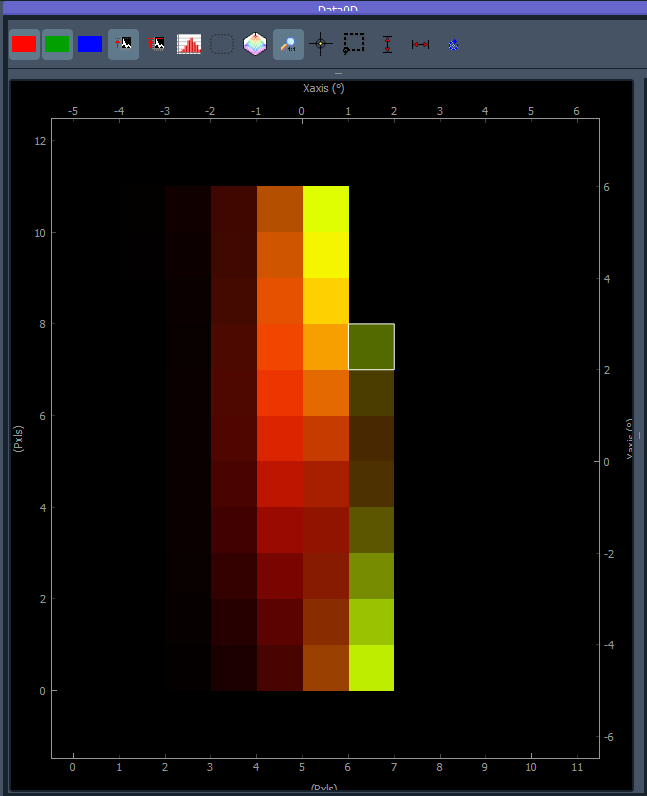
Fig. 3.26 An example of a detector exporting 0D live data plotted as a function of the 2 actuators’s position. Integrated regions of channel CH0 are plotted in red and green.
So at maximum, 2D dimensionality can be represented. In order to see live data from 2D detectors, one should therefore export lineouts from ROIs or integrate data. All these operations are extremely simple to perform using the ROI features of the data viewers (see Plotting Data)
3.5.1.4. Various settings
3.5.1.4.1. Toolbar
The toolbar is comprised of buttons to start and stop a scan as well as quit the application. Some other functionalities can also be triggered with other buttons as described below:
 : will shut down all modules and quit the application (redundant with: File/Quit menu)
Init. Positions: will move all selected actuators to their initial positions as defined by the currently set scan.
 : will start the currently set scan (first it will set it then start it)
 : stop the currently running scan (in case of a batch of scans, it will skips the current one).
 : when checked, allows currently actuators to be moved by double clicking on a position in the live plots
 : opens the logs in a text editor
3.5.1.4.3. Settings
The settings tree as shown on Fig. 3.20 is actually divided in a few subtrees that contain everything needed to define a given scan, save data and plot live information.
3.5.1.4.3.1. General Settings
The General Settings are comprised of:
Time Flow
Wait time step: extra time the application wait before moving on to the next scan step. Enable rough timing if needed
Wait time between: extra time the application wait before starting a detector’s grab after the actuators reached their final value.
timeout: raise a timeout if one of the scan step (moving or detecting) is taking a longer time than timeout to respond
Scan options :
N average: Select how many scans to average. Save all individual scans.
Scan options : * Get Data probe selected detectors to get info on the data they are generating (including processed data from ROI) * Group 0D data: Will group all generated 0D data to be plotted on the same viewer panel (work only for 0D data) * Plot 0D shows the list of data that are 0D * Plot 1D shows the list of data that are 1D * Prepare Viewers generates viewer panels depending on the selected data to be live ploted * Plot at each step
if checked, update the live plots at each step in the scan
if not, display a Refresh plots integer parameter, say T. Will update the live plots every T milliseconds
Save Settings: See h5saver_settings
3.5.1.4.3.2. Saving: Dataset and scans
DAQ_Scan module will save your data in datasets. Each dataset is a unique h5 file and may contain multiple scans. The idea behind this is to have a unique file for a set of related data (the dataset) together with all the meta information: logger data, module parameters (settings, ROI…) even png screenshots of the various panels.
Fig. 3.27 displays the content of a typical dataset file containing various scans and how each data and metadata is used by the H5Browser to display the info to the user.
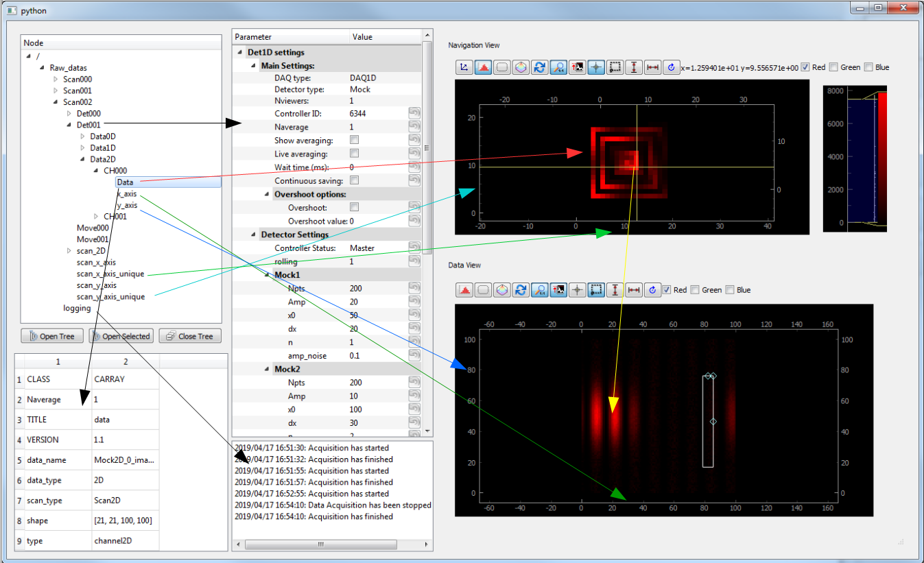
Fig. 3.27 h5 browser and arrows to explain how each data or metadata is being displayed
The Save Settings (see Fig. 3.28) is the user interface of the H5Saver, it is a general interface to parametrize data saving in the hdf5 file:
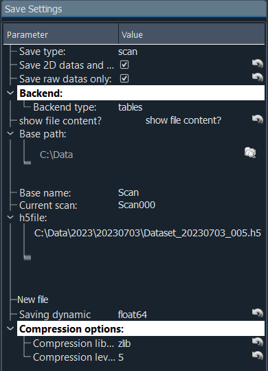
Fig. 3.28 Save settings for the DAQ_Scan extension
In order to save correctly your datas, saving modules are to be used, see Module Savers.